Overview
This is an OSLO tutorial about ray tracing with mirrors. It is builds on the previous mirror tutorial and that you understand the skills taught there.
This follows the mirror tutorial created Brian Blanford in 2009.
This tutorial is one from a list of other tutorials that are available.
The FAQ might also be of help.
New ideas:
Displaying spot diagrams and an Airy disk
Displaying point spread function (PSF) and Strehl ratio
Paraxial focus, RMS focus, and OPD focus
Off axis rays
Adding an aperture to minimize coma
Bending the image surface to minimize off axis errors
f/4 Telescope
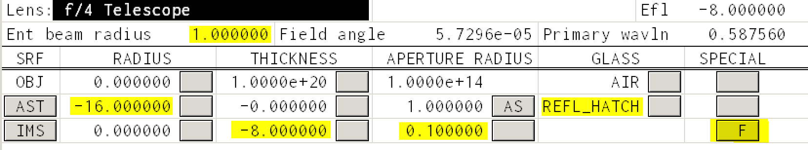
Let's model a f/4 reflecting telescope having a concave mirror with a radius of curvature of 16mm. First, we need to figure out where the image will be and what the diameter $D$ of the mirror will be.
Recall that $$ f= \frac{R}{2} $$ and so for this mirror the image surface will be 8mm away from the mirror.
The f/# is the focal length divided by the limiting aperture $$ f\# = \frac{f}{D} $$ therefore the diameter of the mirror will be 2mm (and the radius will be 1mm).
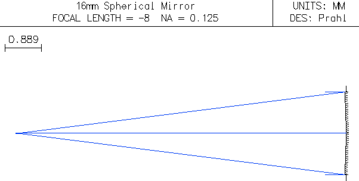
And the drawing should look like
The Spot Diagram
In OSLO, the rays are launched from the source and propagate to the image plane. The spot diagram shows where these rays intersect the image plane. This is useful for evaluating an optical design.
Go to the menu item
Evaluate -> Spot Diagram -> Single Spot Diagram
and change the setting to show the Airy disk. The Airy disk is the diffraction limited spot or more simply the smallest spot that could possibly be achieved for this system.
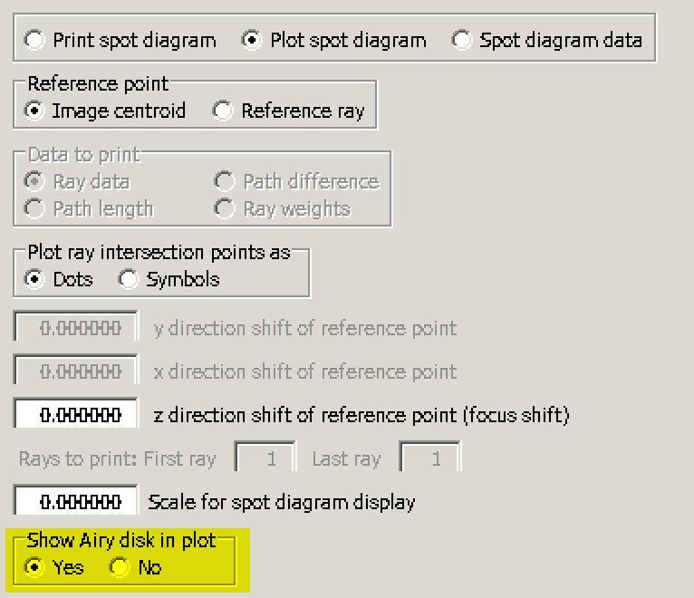
You should now see
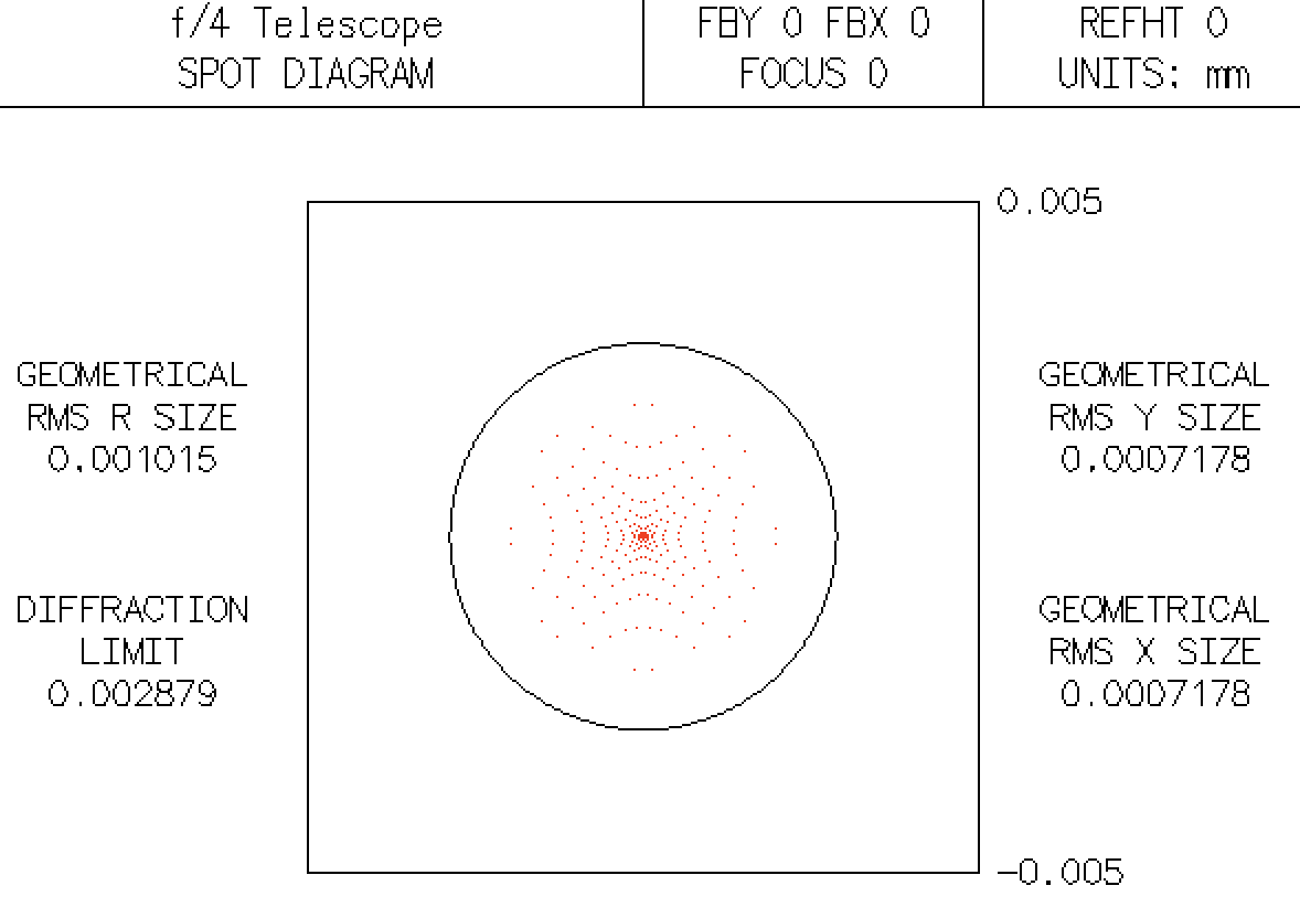
The circle represents the Airy disk and since all the small points fall within the circle, we can say that this f/4 telescope is diffraction limited.
In this case we can validate the Airy radius using $$ r_{Airy} = 1.22 \frac{\lambda f}{b} $$ where $\lambda=587.56$nm, $f=8mm$ and $b$ = 2mm.
lambda0=587.56e-9          # m
f = 8e-3                   # m
b = 2e-3                   # m
r_airy = 1.22*lambda0*f/b  # m
print("The diffraction limited spot size is %.5f mm" % (r_airy*1000))

print("entering beam radius should be %.2f mm" % (8/2.33/2))
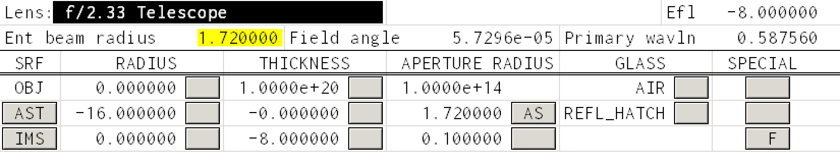
What about a f/2.33 telescope?
In this case, the limiting aperture increases to $$ d = \frac{f}{f/\#} = \frac{8\mbox{ mm}}{2.33}= 3.43\mbox{ mm}. $$ and the entering beam radius should now be set to 1.72mm.
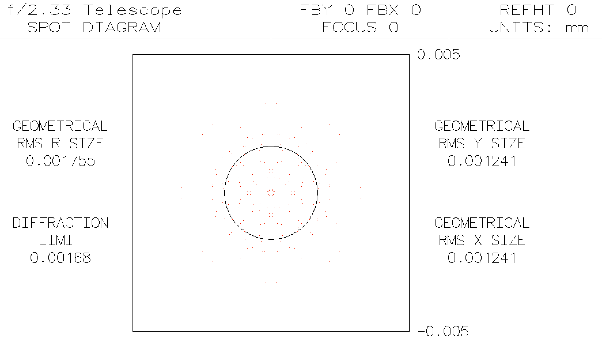
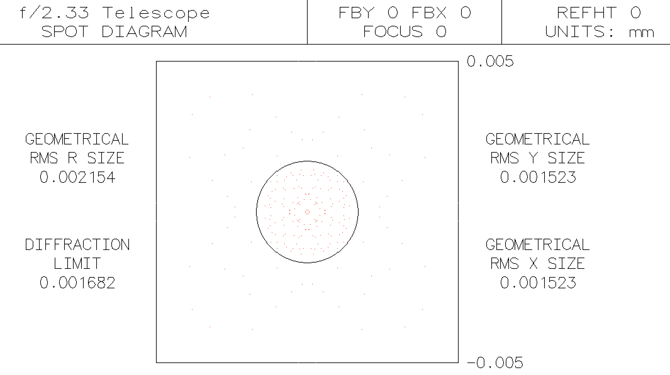
Set the entering beam radius and bring up the single spot diagram again to see that many points now fall outside the Airy disk
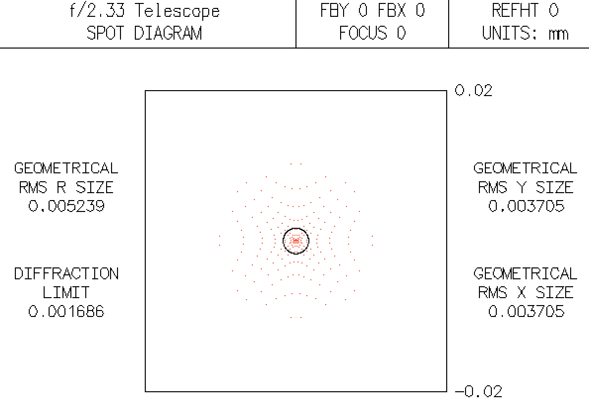
This is no longer diffraction limited — or is it?
Better focusing 1
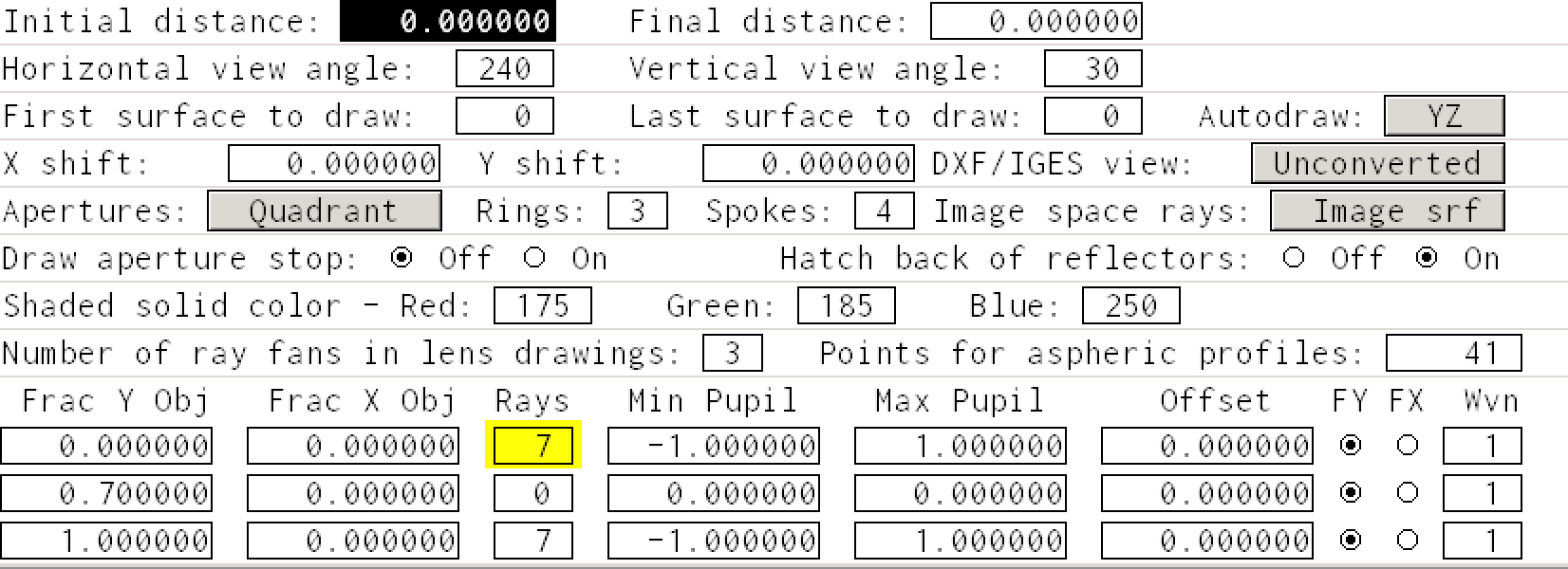
First, let's add a few extra rays to the ray drawing by going to menu
Lens -> Lens Drawing Conditions ...
and increasing the number of rays drawn from 3 to 7.
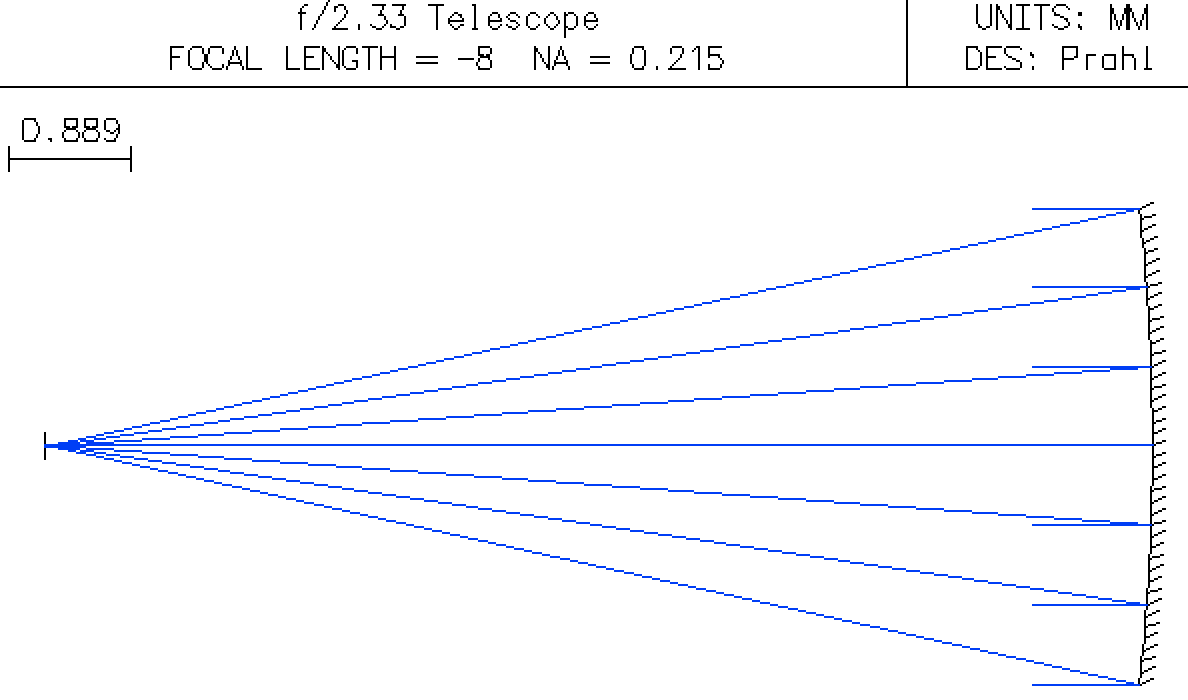
If we look at the focusing of the mirror in the default autodrawing image, it looks just fine.
The Autofocus window cannot be zoomed. However, it is possible to zoom using the UW 1 Window. Do this by clicking the first icon in the UW 1 window and selecting Lens Drawing. You should now see a new row of icons,
Click on the second icon in theUW 1 menu and the Autodraw image will be repeated. However this window allows you to click drag a rectangle to zoom into a region of interest. If you zoom into the region around the focus you see
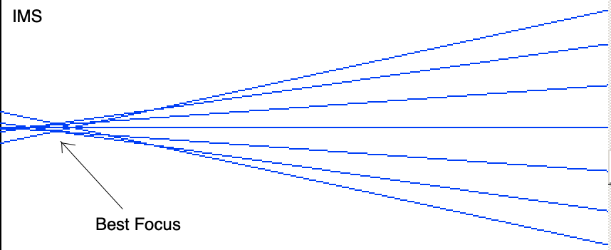
Now it is clear that the best focus does not coincide with the image surface IMS. It would improve the focus if we move the IMS back towards the mirror. The easiest way to do this is to click on the button in the thickness column in the IMS row and select
Autofocus - Minimum RMS Spot Size -> On-Axis Monochromatic
The thickness should change to -7.968223. Now generate a
Now, most points fall within the Airy disk!
However, to quantitative assess whether the system is diffraction limited, the Strehl ratio is commonly used. Generally, a Strehl value above 0.8 represents a diffraction limited spot.
The easiest way to display the Strehl ratio is to go to the UW 1 Window and click the first icon in the UW 1 window and selecting Lens Drawing. You should now see a new row of icons,

Select the third icon
The number in the upper right hand corner is the and represents how close to perfect the optical system is. The value of 0.5454 says that the spot is not diffraction limited.
Better focusing 2
If instead we select the other option
Autofocus - Minimum OPD RMS -> On-Axis Monochromatic
to minimize the root mean square optical path difference. In this case, the thickness should change to -7.976253 and the spot diagram looks like it might be a bit better:
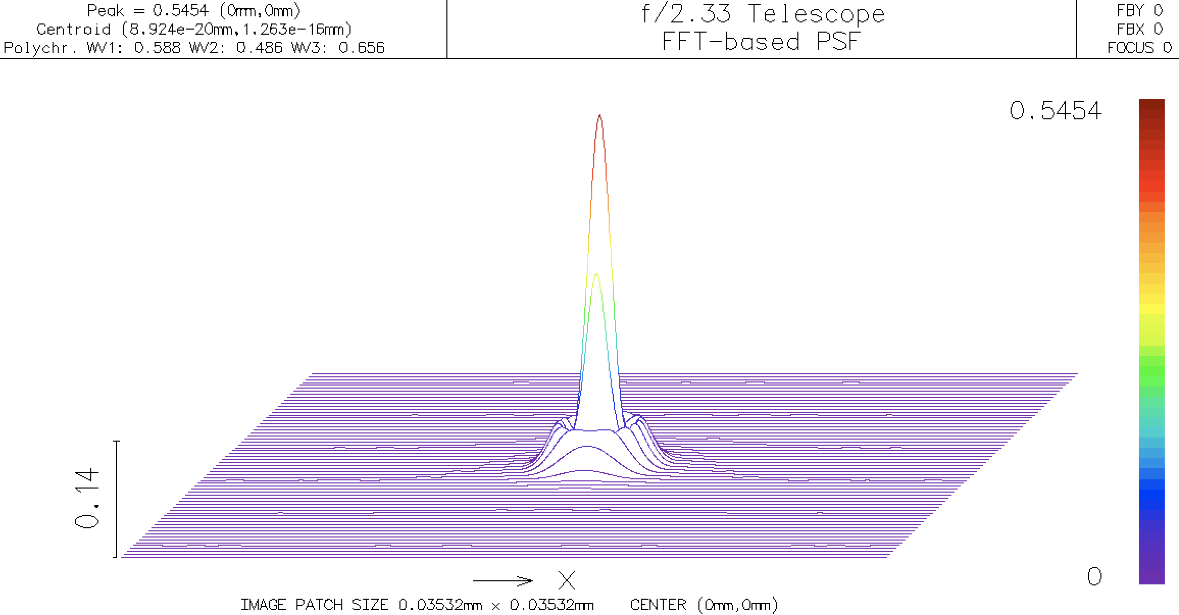
Now when we look at the point spread function, we see a new Strehl ratio
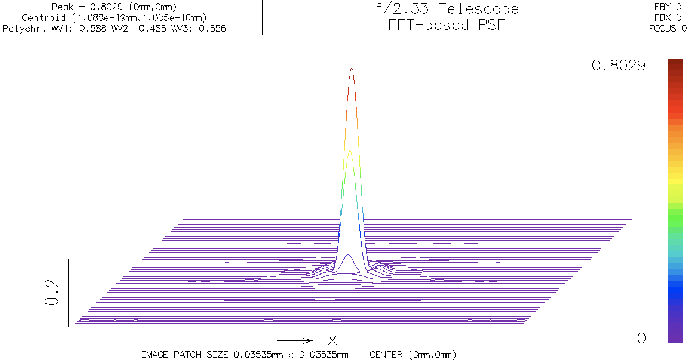
And we see that the telescope is (barely) diffraction limited because the Strehl ratio is now since 0.8029.
Off-Axis Behavior
So, the mirror works as well as can be expected for paraxial rays, even at f/2.33 now. A good telescope should allow one to focus on stars adjacent to those in the center of the field. To do this, we will increase the field angle to ±18°.
To continue, at the moment, just go to page 13 of Blandford's mirror tutorial.
The steps are
- insert a new surface 1
- make it the aperture stop
- make its position variable
- create sliders to optimize the stop location and mirror curvature
Eventually, you will discover that the best place for the aperture stop is at the center of curvature of the mirror.