OSLO - Landscape Lens - Basic Iteration¶

Scott Prahl

Sep 2019, Version 1

This follows one of the official OSLO tutorials pretty closely. I do try to add context (and opinion) that I felt was missing from the original tutorial.

Overview¶

This is the third tutorial that covers OSLO basics. In this tutorial, OSLO will be configured to automatically adjust a surface radius to achieve a specific focal length.

The FAQ may give you a hint or two that will make the OSLO experience a bit less horrible.
The first part should have gotten you to the point of entering most of the lens data into the Surface Data spreadsheet.
This second part explains how to set the size of the object and select rays to be traced.
This tutorial is one from a list of other tutorials that are available.

New ideas¶

Creating an empty aperture/stop
Using a standard optical glass N-BK7
Using Autofocus - paraxial focus
Using OSLO to automatically optimize a design
Making a lens parameter Variable
Defining an error to minimize

Landscape Lens Design¶

Ansel Adams took the picture below at Glacier National Park. His camera needed a lens that captures a wide field-of-view (FOV). A lens with both a wide FOV and small aperture is called a landscape lens. (Aperture and field size together determine the difficulty of an optical design, so allowing the aperture to be small makes the design easier.)

So what what exactly is a landscape lens? Bentley writes

Landscape photography requires wide-FOV lenses that capture as much of the scenery as possible. Shifting the stop in a singlet away from the lens increases its FOV and results in a simple landscape lens. ... The farther the aperture stop is shifted from the lens, the larger the lens diameter. Disposable “box” cameras generally use simple landscape lenses.

where stop refers to limiting aperture AST. Basically, we are allowed to reduce the size of the stop move it around in our design. She also writes:

As the stop is moved, the lens shape changes and is generally bent around the stop to reduce the ray angles of incidence and the off-axis aberrations. The stop shift also introduces astigmatism that helps to flatten the tangential field curvature. A single-element landscape lens still has spherical aberration and chromatic aberrations and is therefore restricted to a small NA.

which probably makes no sense to you at the moment. We will return to this later once we have introduced a few more ideas.

The goal is to develop a cheap singlet with a focal length of 100mm and a field-of-view of ±20°

Starting Design¶

Landscape photos have objects that are generally far away. The best starting lens shape will be a plano-convex lens with the curved side oriented towards the objects --- because this will bend more or less equally on both surfaces. We will use N-BK7 glass because it is the cheapest glass available. For a plano-convex lens, a initial radius of curvature of 50mm will get us pretty close to a focal length of 100mm.

This means our starting parameters will be

Plano-convex lens made of N-BK7 glass
Radius of curvature of first lens surface of 50mm
Lens thickness of 4mm
Field-of-view of ±20°
Entering beam radius of 10mm
Add a stop 10mm behind lens

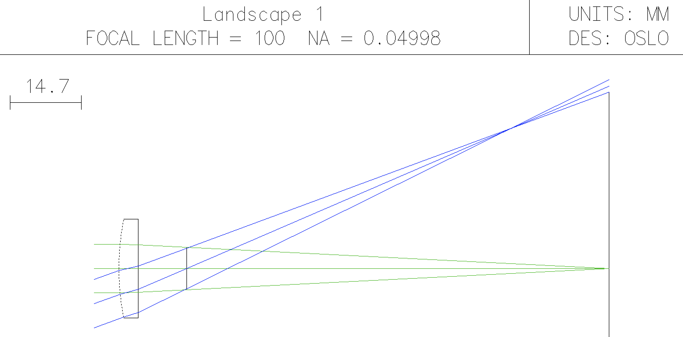
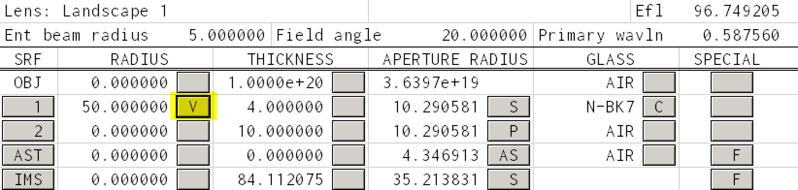
For now, we will leave the diameters of the aperture stop and lens unspecified (OSLO will solve for these automatically). Once the lens has been entered, you should have the drawing above and the following spreadsheet

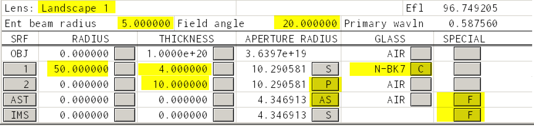
You will need to do something with every one of the yellow areas in the dialog above. Note that

the glass is changed to N-BK7 by either typing directly or selecting from the Catalog->Schott dialog
the third row is set to AST (using the button under APERTURE RADIUS)
the APERTURE RADIUS button for surface 2 is set to Pickup from surface 1
both the AST and IMS have Surface Control set to Drawn in the last column

You should end up with something that looks like this:

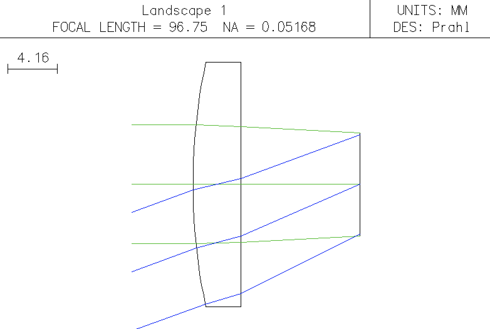
Notice how the rays at 0° and at 20° both cross exactly in the plane of the aperture stop AST.

Tracing rays to the image surface¶

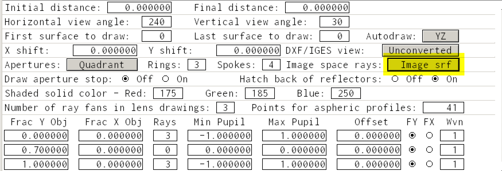
Now, in the image surface can be easily located at the paraxial focus using the button in the thickness column and selecting Autofocus - paraxial focus. Unfortunately, nothing changes in the Autodraw window. This is perplexing because we have already selected Drawn for the IMS row.

In this case we need to use dialog box found using the menu item Lens->Lens Drawing Conditions. Specifically, change the Image space rays: button to Draw to image surface and it will display Image srf

And the Autodraw window will become

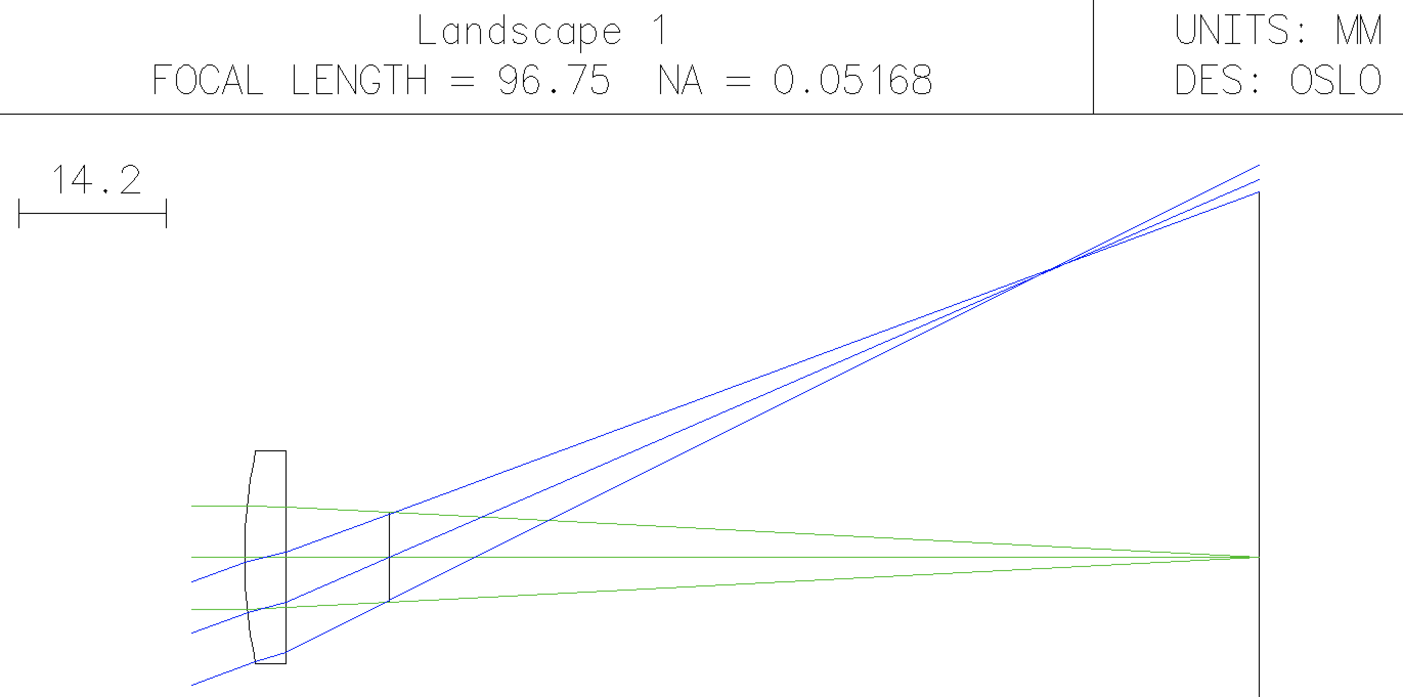
which shows that the large angle rays are poorly focused in the image plane. A good landscape lens will have the paraxial rays and the off-axis rays focused to a single point.

Fixing the focal length manually¶

Well, we can do what we did before. Specifically, change the radius of curvature of the first surface manually. Type a number in, see what the EFL is and repeat until the EFL is 100mm.

the desired focal length is longer than 96.75 and therefore the radius of curvature needs to be greater than 50 so light is bent less

With a couple of guesses, you should obtain

So far, so good. However,

we would like the program to do this for us
we would like to minimize coma as well

Change the radius of curvature back to 50mm.

Fixing the focal length automatically¶

We need to do three things

tell OSLO what can be varied
tell OSLO what error should be minimized
tell OSLO to iterate

The parameter to be varied¶

The first is really easy. Just mark the radius of curvature of the first surface as variable

Defining the error¶

Defining the error can be an elaborate process. However, we just want OSLO to set the EFL to 100mm. To do this we select the menu item

Optimize -> Generate Error Function -> Aberration Operands

and change the three entries shown below

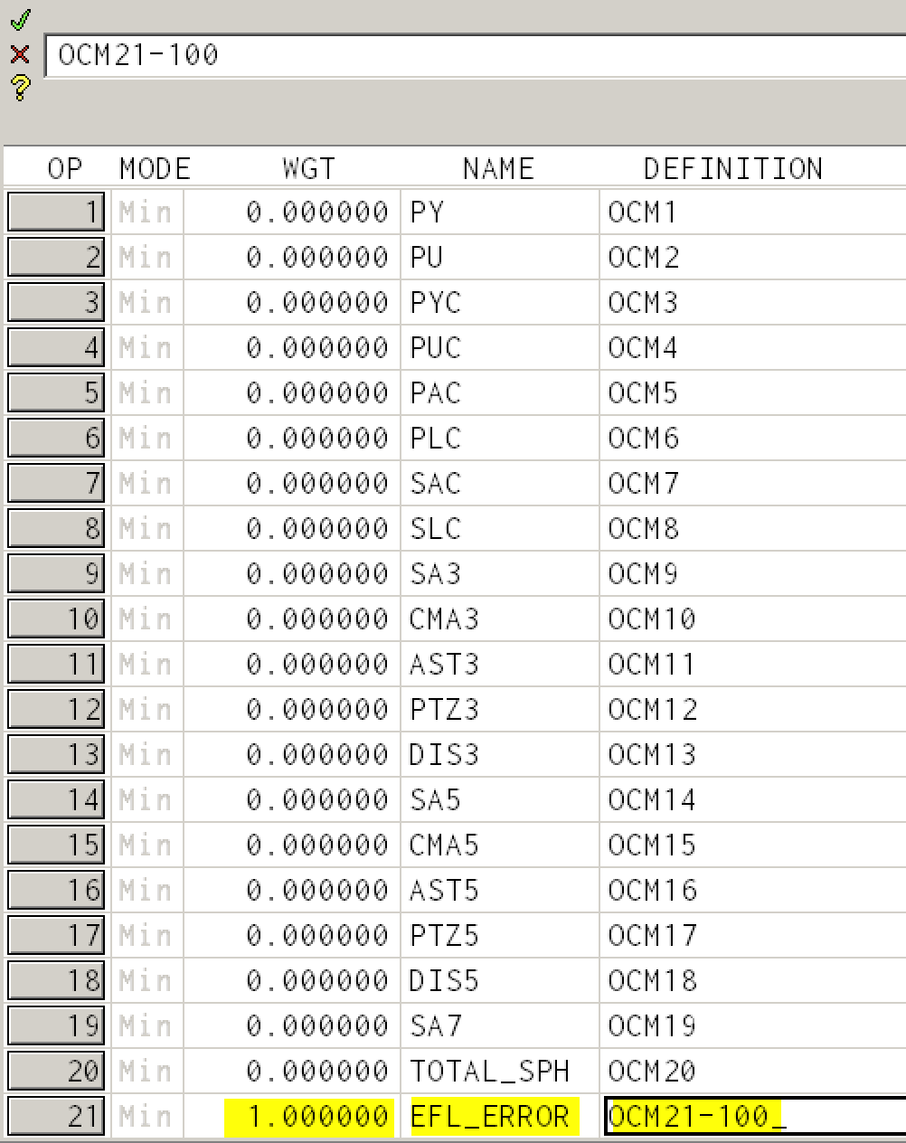
The first column is the weighting or emphasis to place on a particular source of error. Since we only care about the EFL, we the entire contribution to come from this line and we set the value to 1.0. (All the other lines are ignored because their weights are zero; only line 21 matters now.)

The second column is a name for the parameter that is being minimized. We rename the line to EFL_ERROR for clarity. Unsurprisingly, this line will represent the "error in the effective focal length". Non-zero values of EFL_ERROR indicate that the automatic minimization process is not finished.

The third column is how the variable EFL_ERROR will be calculated. Since the internal OSLO variable named OCM21 is equivalent to the EFL, we want OCM21-100 to be zero.

In this way, we have defined an OSLO error function that will be zero when the EFL=100.

Iterating¶

Select the menu item

Optimize -> Iterate

and click OK. (If the Iterate item is not functional, make sure that you have defined the curvature of surface 1 as "Variable" and have defined your error function as discussed above.)

After you ask OSLO to manually paraxially focus the image surface again (via the button in the THICKNESS column of the IMS row), you should obtain

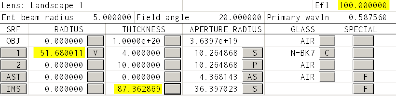
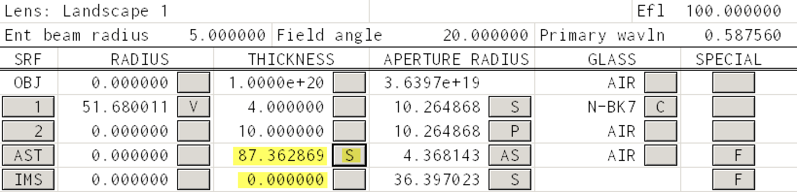
The highlighted entries show that the EFL is now 100mm.

Avoiding the need to focus manually every time¶

Clicking a button to focus is something that OSLO should do for us. So let's first set the THICKNESS of the IMS surface to zero.

Now click the button in the THICKNESS column of the third surface (AST) and select

Solves -> Axial Ray Height

In the dialog box that appears enter a solve value of zero. OSLO will then figure out the distance so that the paraxial chief ray intersects the optical axis (an axial height of zero).

Your final lens spreadsheet should look like

Next steps¶

The next tutorial. will explore improving this lens to minimize comatic aberration.

This tutorial is also available in the form of a Jupyter notebook.

The final OSLO lens file for this landscape lens can also downloaded.