Now that you know how to get access to the code. I found little difficulty following the program; even though, I've never seen a line of C code before in my life. Any good C reference should make the code readable without taking up your afternoon. One should find that the code will compile without complaint. I did get one warning message using CodeWarrior, about a missing return value at the end of the program, but this can be ignored. The compiled code runs quickly spitting out an easy to interpret data file, which can be utilized in a variety of other programs (e.g. Excel or KaleidaGpraph). Any of the optical parameters are easily changed to fit as a model for your experiments. Each optical parameter is listed in the beginning of the program as a variable, which is clearly documented. Also to alter the separation between data points, simply changing the shell thickness.
The Tiny Monte Carlo program is very simple to use and produces realistic data. And best of all, one does not need to be the brightest kid on the block to make it work for you. The program outputs data that agrees well with diffusion theory. I did a quick comparison using Akira Ishimaru's expression for the diffusion equation for the same boundary conditions:
where the solution for the average diffuse intensity is
P0 is the total radiant power. However, a more common notation for Ishimaru's other variables may be given by
where µa, µs', and µt' are the absorption coefficient [cm-1], the reduced scattering coefficient [cm-1], and the total attenuation coefficient [cm-1] respectively. By making the above substitutions and solving for the heat, heat[Wcm-3] = Ud µa , it follows that
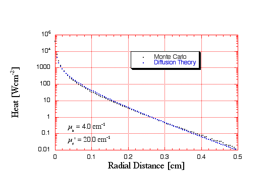
The graph below compares the Teensy Monte Carlo results to this diffusion theory equation. I ran these comparison graphs for various different optical parameters; The program defaults for these parameters are µa = 2.0 cm-1 and µs' = 20.0 cm-1. The agreement between the program and the diffusion theory all were very similar to the one shown.
