The basic Monte Carlo technique

This section describes how the computer uses a random number generator to sample in an unbiased fashion values of a parameter x from a particular probability density function, p(x). In other words, if a large number of rnd values were used to choose a large number of x values and these choices of x were plotted as a histogram, the shape of the original p(x) would be reconstructed.

The computer's dice

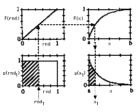
The computer has a random number generator which can yield a random number, rnd, between 0 and 1 each time the computer calls that subroutine. This rnd is the computer's dice. The probability density function, p(rnd), is uniformly distributed between 0 and 1 with an assigned value of 1. The probability distribution function, F(rnd₁), is defined as the integral of p(rnd) over the range of 0 <= rnd <= rnd₁, and linearly increases from 0 to 1 as rnd₁ increases from 0 to 1.

The desired p(x)

Suppose that we are interested in a probability density function, p(x), that describes the likelihood of the parameter x taking on a specific value, perhaps the specific value x₁, between the limits a and b: a <= x <= b. The probability distribution function, F(x₁), is defined as the integral of p(x) over the range of a <= x <= x₁, and increases from 0 to 1 as x₁ increases from a to b.

The connection between rnd and x.

The key to the Monte Carlo technique is to recognize that if one lets F(rnd₁) equal F(x₁), then a point of connection is made between p(rnd₁) and p(x₁). Random selection of rnd maps into a distributed selection of x that mimics the original p(x).

The following figure illustrates the connection between p(rnd₁) and p(x₁) via the equation of F(rnd₁) equal F(x₁):

click on figure to enlarge

A random number, rnd1, is chosen by the computer. The value rnd1 points to a value F(rnd1). The value F(rnd1) points to an equal value F(x1). The value F(x1) points to a value x1. This process is equivalent to equating the hatched areas under the p(rnd) and p(x) curves in the figure. The total areas under the p(rnd) curve from 0 to 1 and under the p(x) curve from a to b are both equal to 1. In this way, a choice of rnd1 chooses a unique value x1. As a large number of random numbers, rnd1, are chosen, the set of associated x1 values will be sampled from p(x) in a non-biased way such that the histogram of chosen x1 values will mimic the original function p(x).

Mathematically, the equivalence of F(rnd₁) equal F(x₁) can be stated as:

or more simply:

After evaluation of the integral above, the expression can be rearranged to solve for x₁ in terms of rnd:

This expression function(rnd) can then be used to specify a choice of x for each random number, rnd, generated by the computer's random number generator. That's it!