OMLC
the library
NewsEtc
the blog
steve
|
ABSTRACT |
INTRODUCTION In optical studies, we often prepare mixtures that optically mimic biological tissues, which we call "phantom" tissues. These phantoms allow us to test optical devices or evaluate the dosimetry of therapeutic protocols using light. This article describes how to prepare and calibrate a phantom.
METHOD
Prepare a phantom Take a cup of milk and add some colored juice. Call this our "phantom" tissue. Let us calibrate this mixture to specify its optical properties.
Setup the calibration experiment Set up a light source so that it illuminates either the center of the cup or a reflectance standard. Figure 1A shows a cup illuminated by an optical fiber delivering white light that is refocused by a lens to a point on the milk surface. A detector fiber views the total surface of the milk from a distance. Figure 1B shows the same setup with a reflectance standard. The position of the standard's surface matches the position of the milk's surface.
A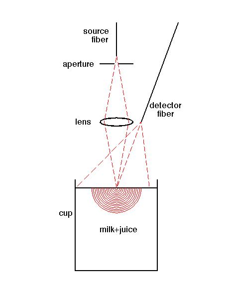 B
B
Fig. 1: Experimental setup. (A) White light illumination from a source fiber illuminates the milk mixture at a point. Escaping reflectance is sampled by a detector fiber that carries light to a spectrometer. (B) Same measurement, but phantom is replaced by a reflectance standard of known refledtance Rstd.
Let the cup be sufficiently big that when you illuminate the center of the surface of the milk with a point of light (the focused white light source) the light will spread out but not touch the edges of the cup, nor the bottom of the cup. The cup holds 500 ml milk + juice.
Added Absorber Experiment
Step 1: Measure the standard --> Mstd in arbitrary lab units.
The spectrometer measures the spectrum of light intensity collected by the detector fiber, which reflected from the reflectance standard: Mstd [counts/bin].
Step 2: Measure unknown mixture --> Msample
The spectrometer measures the spectrum of light intensity collected by the detector fiber, which reflected from the unknown sample: Msample [counts/bin].
Step 3: Measure unknown mixture + added absorber --> Msample+Δµa
Add one ml of known absorber (1ml of stock with µa stock = 1000 cm-1), and measure: Msample+Δµa [counts/bin].
The added absorber in the milk is equal to (1000 cm-1)(1 ml/501 ml) = 1.996 cm-1. In preliminary experiments, the µa stock of the stock absorber was determined by measuring transmission through a 1/1000th dilution of the stock in a 1-cm-pathlength cuvette. The transmission, relative to a blank cuvette filled with water, was T = Mdiluted stock/Mblank = 0.3679. Hence, µa stock = -ln(0.3679)/(1 cm)/dilution = (1 cm-1)/(1/1000) = 1000 cm-1.
Step 4: Calculate reflectances --> Rsample and Rsample+Δµa
Rsample = RstdMsample/Mtd
Step 5: Calculate optical properties --> µa and µs' = µs(1-g)
The are several methods to do the calculation. This article uses a graphic method to illustrate the process, and an interpolation algorithm (written in MATLAB) to calculate routinely.
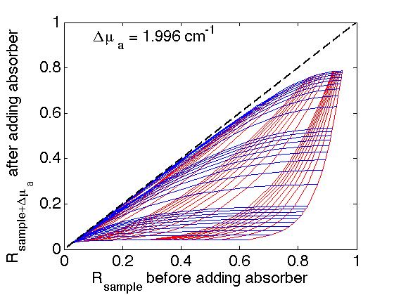
| Graphic analysis grid Use a transport model to calculate the reflectance from a semi-infinite medium of refractive index n = 1.33 and an air/water interface. This model can be called getRd(µa, µs',n). It can be a Monte Carlo model, or diffusion theory, or some implementation of radiative transport theory. For this article, we use a simple approximation for n = 1.33, listed here: getRd.m. Create an analysis grid by sequentially calculating Rd for a matrix of choices of µa and µs'. For example, choose µa = [0.01:0.01:0.1 0.2:0.1:1 2:1:10 20:10:100], a logarithmic range between 0.01 to 100 cm-1 µs' = [1:1:10 20:10:100 200:100:1000], a logarithmic range between 1 to 1000 cm-1 Calculate the values of getRd(µa, µs') and plot the analysis grid. A program to do this is listed, makeGrid.m, which yields Figure 2:
| |
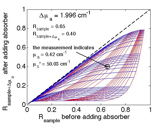
| Interpolation using the analysis grid Interpolation of a pair of measurements Rsample and Rsample+Δµa using the analysis grid is illustrated in Fig. 3, which was created by the program analyzeGrid.m getRd.m.
|