Keynote Address
1stInternational Biophotonics Meeting
in Israel
Dec 9-11, 2012, Tel Aviv University
slide 1
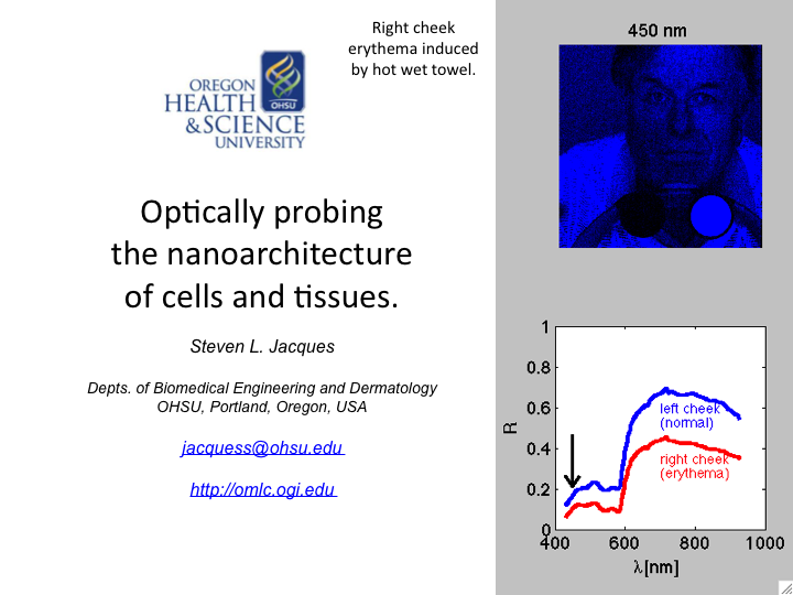
1. This talk discusses how light can probe the nanoarchitecture of cells
and tissues. The emphasis is on the process of light scattering by
tissue structures both larger than and smaller than the wavelength of
light.
slide 2
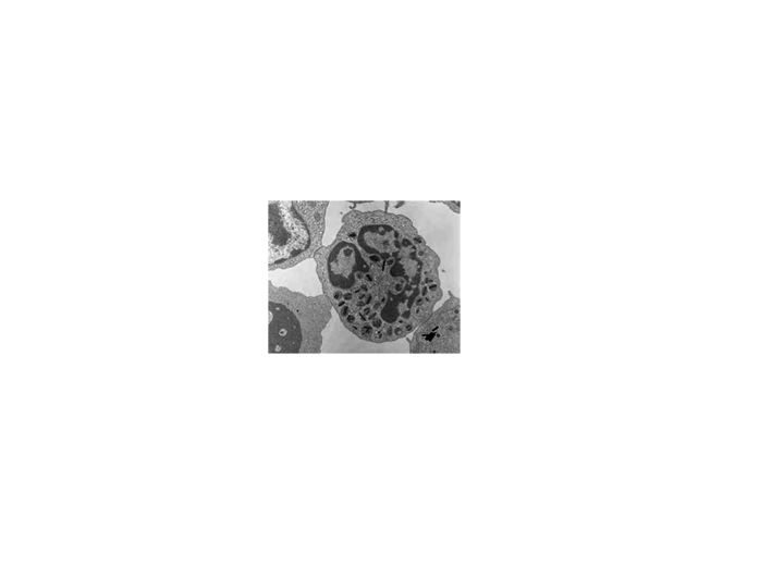
2. This is an electron microscope image of a cell. Note the variety of
sub-cellular structures which are on the scale of a wavelength of light.
Such structures efficiently scatter light.
slide 3
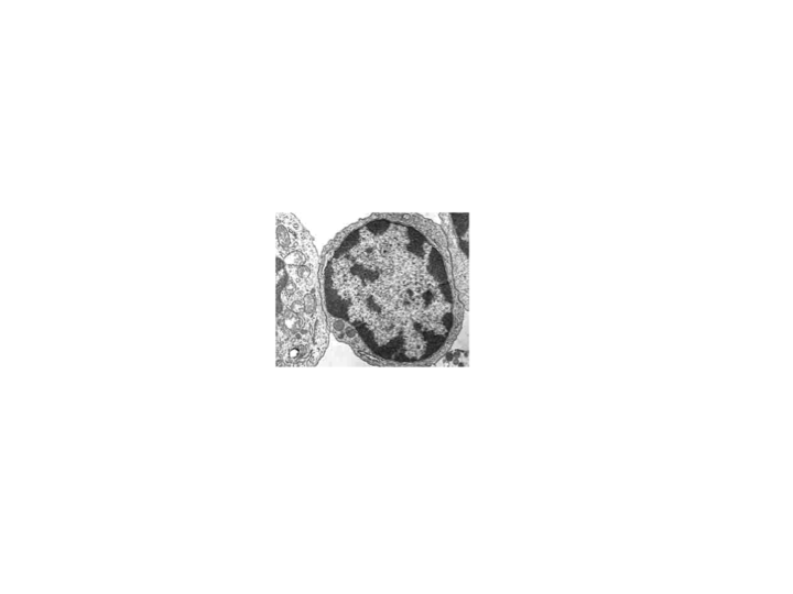
3. This is another EM image of a cell.
slide 4
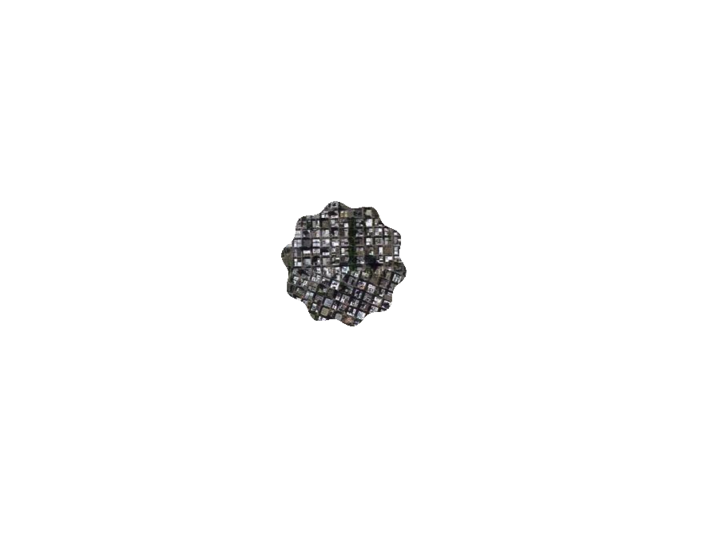
4. This is another image... not of a cell but ...
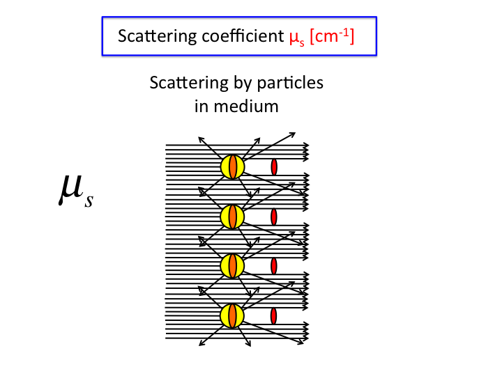
slide 5

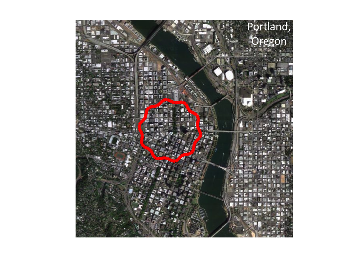
5. ...an image of Portland, Oregon, my home town, as viewed from an
airplane. Note that the distribution of sizes of structures are similar
to the distribution seen in cells. The size distribution is fractal.
slide 6
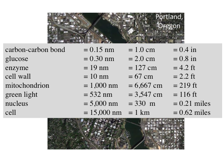
6. On this scale, a carbon-carbon is about 1 cm, glucose fits in the
palm of my hand, and other measures are shown. A cell is like the
downtown area of a city. Green light passing through a cell is like an
ocean wave moving through the city, scattering off cars, buildings,
trees and other structures. From outside the city, optical measurements
can observe the scattered waves and deduce information about the size
distribution of structures within the city/cell that caused the
scattering.
slide 7
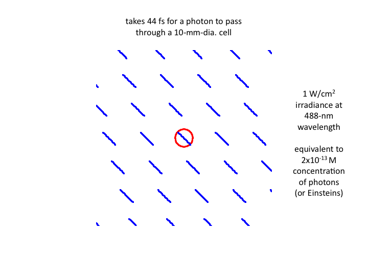
7. Waves of blue light at 1 W/cm2 pass through a cell in
waves, with each wave taking 44 fs to transit the cell. The equivalent
number density of photons is 2x10-13 moles/liter (or
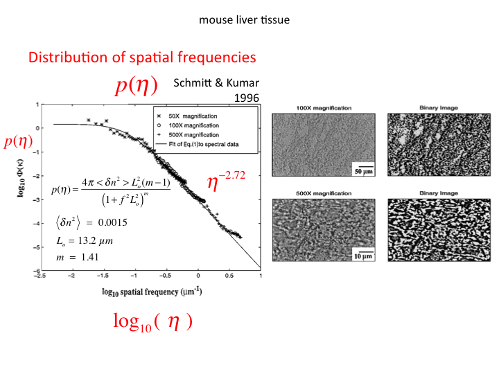
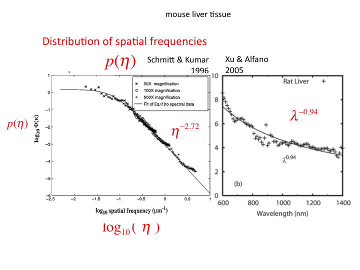
Einsteins).
slide 8
8. Returning to our view of the city/cell, let us move further outward
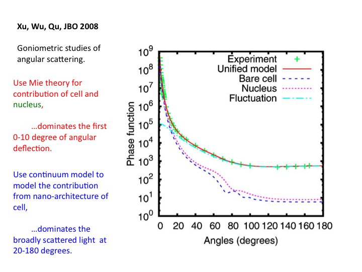
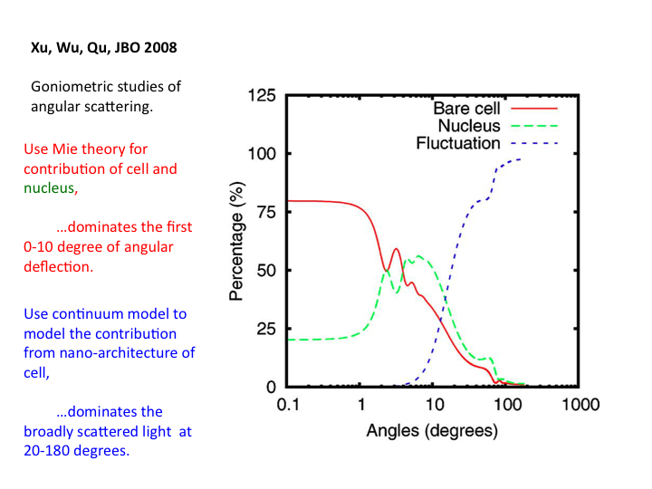
so the cell looks smaller.
slide 9
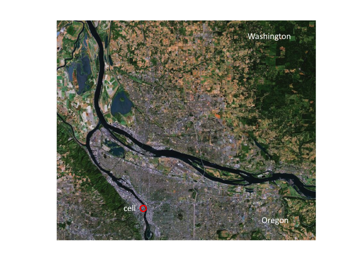
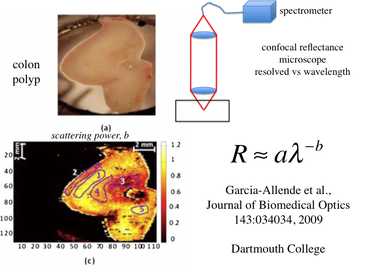
9. Now the cell is a very small part of a larger landscape. In this
picture, the state of Washington is to the north of the Columbia River
and Oregon is to the south of the river.
slide 10
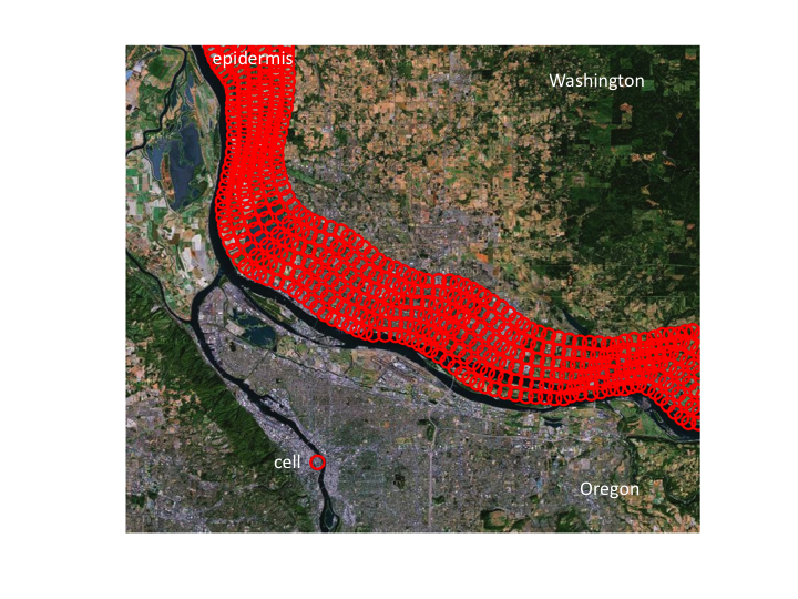
10. An epidermis would appear this thick on this scale.
slide 11
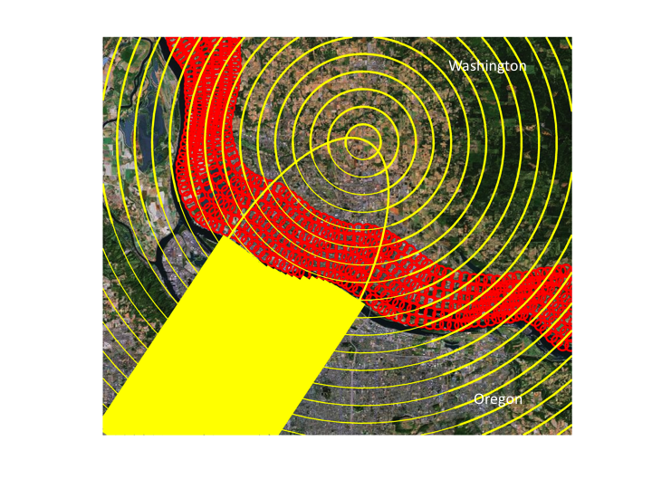
11. If a laser was directed from Oregon into Washington, it would
penetrate through the epidermis into the dermis. It would be possible to
focus the light within the epidermis and the superficial dermis, but by
the time the light reached a depth of 1 transport mean free path (mfp' =
1/(μs(1-g)). shown as the center of circles of diffusion),
the light is sufficiently scattered that it can no longer be focused.
Photons now move down photon concentration gradients.
slide 12
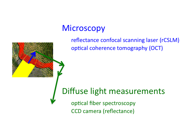
12. Hence, the region with the blue arrow is the domain of microscopy,
while the domain of the green arrows is the domain of diffuse light
measurements.
slide 13
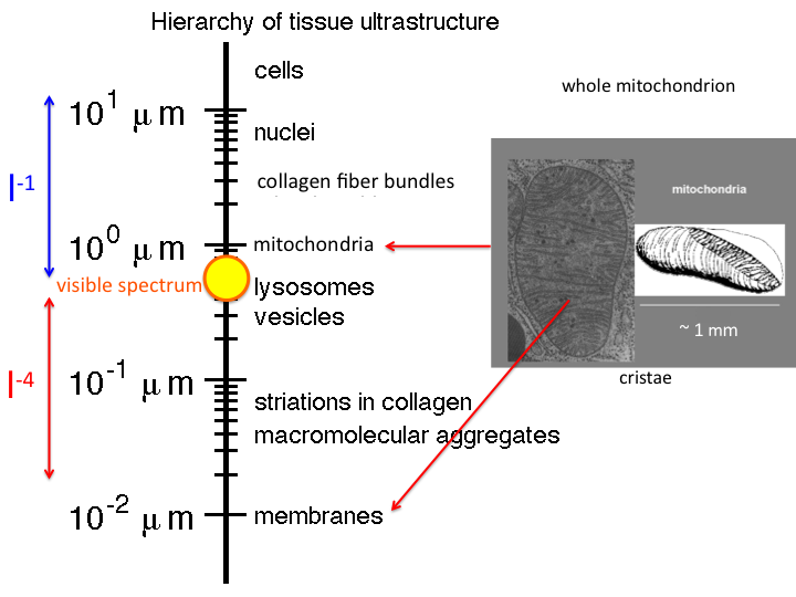
13. There is a hierarchy of tissue ultrastructure, ranging from
membranes (10 nm) to cells (>10 μm). The range of visible light is
shown by the yellow circle. We can easily measure light from about 300 -
1300 nm. Many structures are much bigger than this range of wavelengths,
and scattering by such structures is called "Mie Scattering", which
falls as approximately λ-1. Also many structures are
much smaller than the wavelengths of visible light, and scattering by
such structures is called "Rayleigh Scattering", which falls as
λ-4. Structures like mitochondria present both large
and small structure, and hence contribute both Mie and Rayleigh
scattering.
slide 14
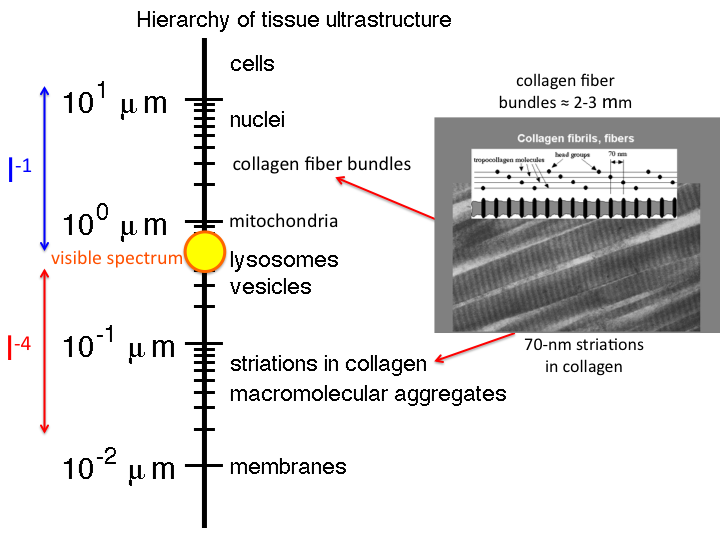
14. Similarly, collagen fibers present both Mie and Rayleigh scattering.
slide 15
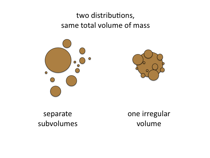
15. In general, cells and tissue present structures which are complex is
shape and are irregularly aggregated. To model the true biological
structure is not possible, but we can "mimic" the optical scattering by
an equivalent "Mie Model" in which a collection of spheres of different
sizes at particular concentrations recreates the optical behavior of the
tissue. Such a "mimic" is a useful metric for characterizing a tissue.
slide 16
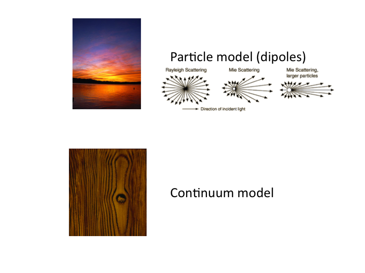
16. There are two approaches toward modeling tissue scattering: (1) the
Mie theory model, which is commonly understood in terms of the blue sky
and red sunset, and (2) the continuum model, which describes the spatial
distribution of refractive index fluctuations, like the grains of wood.
slide 17
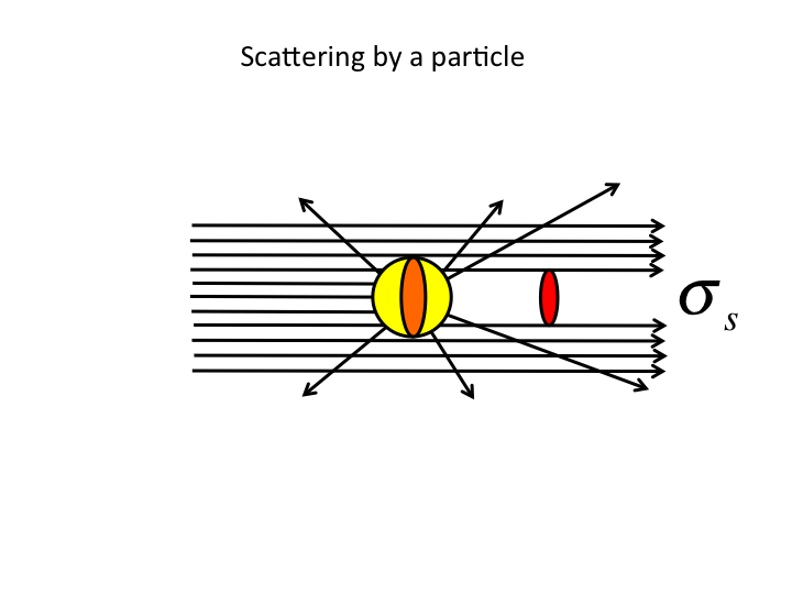
17. First, some definitions of optical scattering properties. The
scattering cross-sectional area, σ [µm2], acts
like a shadow cast by a light-scattering particle.
slide 18
18. Multiplying σ [µm2] by the number density,
ρ [#/µm3], yields the scattering coefficient,
µs [µ-1]. Collimated transmission
through a cuvette of length L [µm] holding a solution of
µs is T = exp(-µsL).
slide 19
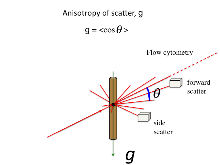
19. When a scattering event occurs, the photon is deflected by an angle
θ. The anisotropy, g [dimensionless], is the average value of
cos(θ).
slide 20
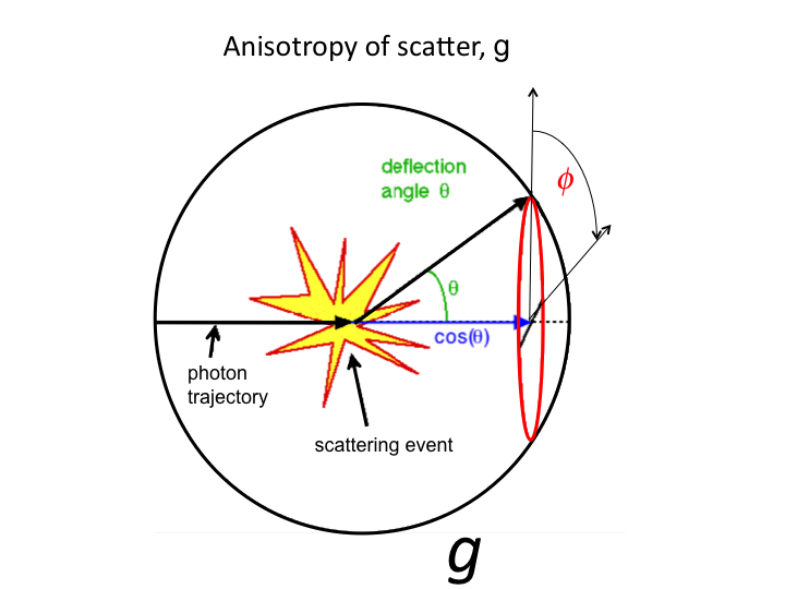
20. The cos(θ) is the projection (blue line) onto the original
axis of photon propagation. Light scatters both forward and backward.
The average value g = <cos(θ)> characterizes the
effectiveness of scattering. As g approaches 1.0, the light is so very
forward scattered that scattering is not so effective.
slide 21
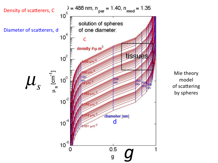
21. If we use Mie Theory to plot all possible values of
µs versus g using a single size sphere, we get this set
of curves. The red contours show increasing density ρ
[#/µm3]. The vertical blue lines show increasing sphere
diameter [µm]. (The µs is here shown as
[cm-1].) Typical values for cells and tissues lay in the
black box in the upper right of the figure.
slide 22
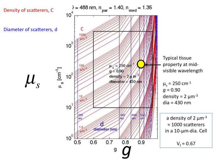
22. This is a close-up of the region were tissue properties lay. The
yellow circle is a typical tissue value in the mid-visible wavelength
range. In other words, a solution of microspheres of diameter 430 nm and
refractive index 1.40 at a concentration of 2 [µm3]
within a solution of average refractive index 1.35 would yield
µs = 250 cm-1 and g = 0.90 at the wavelength
λ = 488 nm (blue light), thereby mimicing the tissue properties.
This concentration corresponds to a volume fraction (vf) of
0.67, at about 1000 scattering spheres per 10-µm-dia. cell.
slide 23
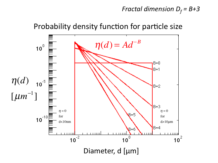
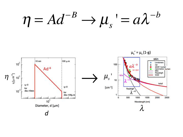
23. Now consider a distribution of sphere sizes, η(d), where d is
the sphere diameter [µm]. The distribution is characterized by a
parameter B. (Often the fractal dimension is cited as Df =
B+3.) The area under each curve is set to 1.0. Artificially, spheres
below 10 nm or above 10 µm are excluded, since the contribution to
scattering from such structures is minor. Scattering is dominated by
structures closer to the wavelength of the light being scattered. As B
increases, the curves become more sloped, having more small scale
Rayeigh scattering and less larger scale Mie scattering.
slide 24
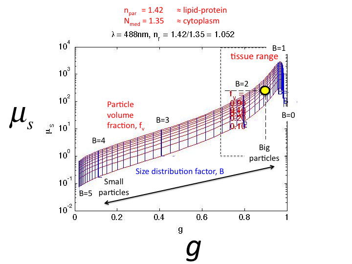
24. Using Mie Theory to calculate the µs and g for
solutions with varying B, the graph shown is generated. The red lines
show constant particle volume fraction, fv = 0.1 to 0.9. The
vertical blue lines show constant values of the size factor B = 0 to 5.
Tissues sit in the black box in the upper right corner. As B decreases,
both µs and g increase.
slide 25
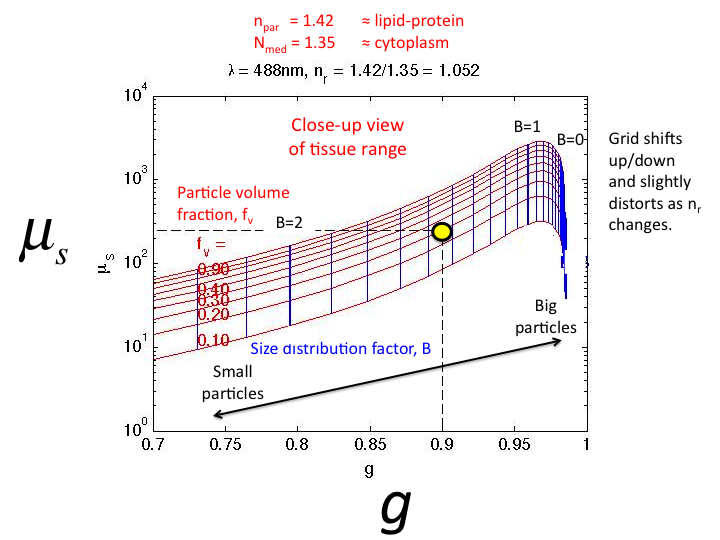
25. A close-up of the tissue region of µs vs g. The
typical tissue value (yellow circle) corresponds to fv = 0.30
(70 percent water) and B = 1.65.
slide 26
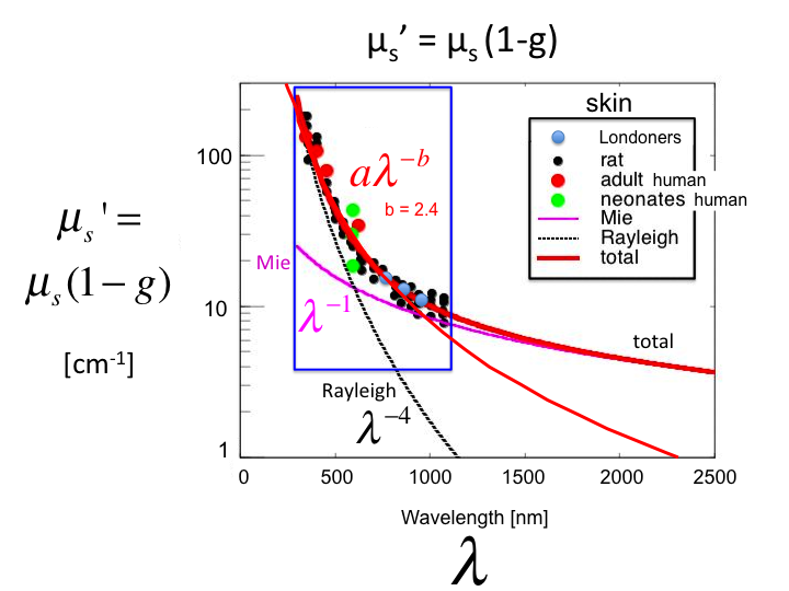
26. A plot of the values of µs' =
µs(1-g) [cm-1] versus wavelength λ
[nm] for skin, based on experiments in humans and rats. The shorter
λ behavior is dominated by Rayleigh scattering
(λ-4], and the longer λ behavior is dominated
by Mie scattering (λ-1]. However, in the region of
practical optical measurements between 300-1300 nm, one can characterize
the behavior by a single parameter b, such that µs' =
aλ-b. In this case, the value of b for skin is 2.4.
slide 27
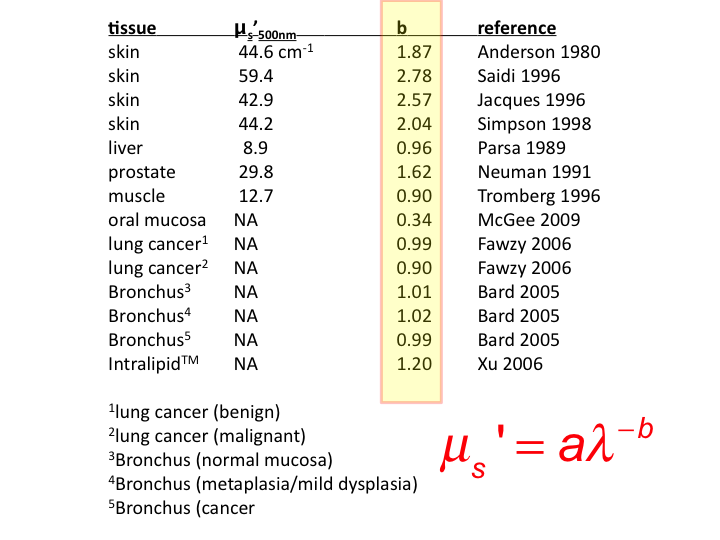
27. The literature cites values of b for various soft tissues and for
skin. Soft tissues show b close to 1.0, while skin values are
slide 28
28. Let us choose a range of B values to predict the properties of
tissue with varying Rayeigh versus Mie scattering, and calculate using
Mie Theory the optical properties versus wavelength,
µs'(λ), then fit the data by
aλ-b to yield a value b that characterizes the tissue.
In this way, we generate the relationship between B and b.
slide 29
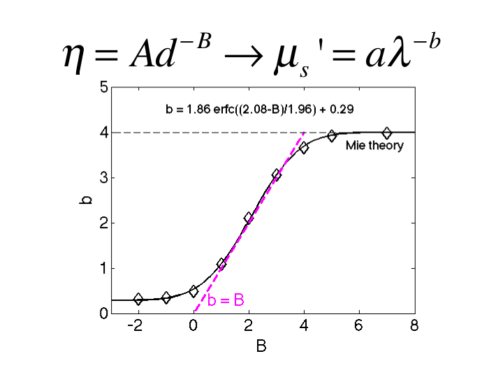
29. This figure summarizes the relationship between B and b. As B
increases to >6, the b approaches 4, consistent with Rayleigh
scattering. As B drops toward 1, the b drops to 1, consistent with Mie
scattering. In the region 1<B<3, the value of b equals the value
of B. This is a convenient relationship appropriate for biological
tissues.
slide 30
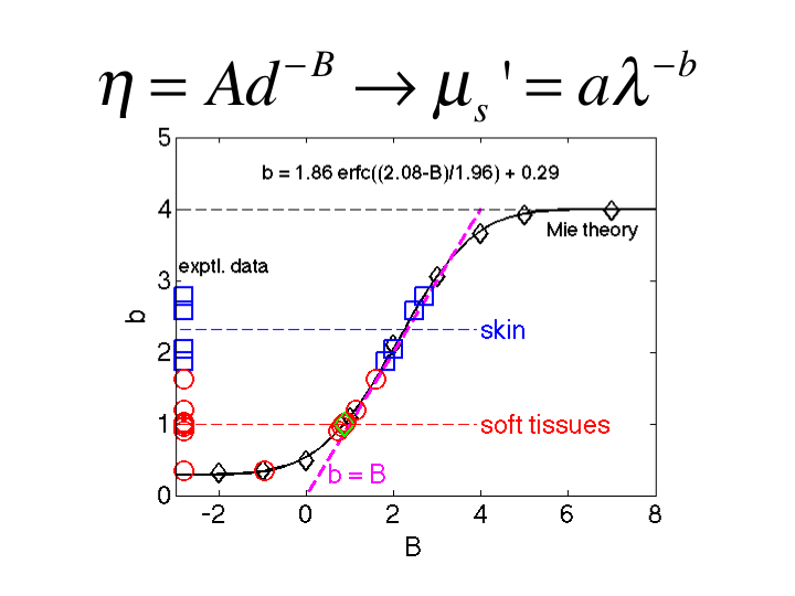
30. Adding the data from the literature, the soft tissue show both b and
B equal to 1.0 and equal to 2 or more for skin.
(NOTE: The
description presented in this talk has not attempted to include the
"packing factor" effect due to close packing of sphere, which generally
lowers the scattering properties due to constructive interference of
scattered waves from the spheres. The "packing factor" is an important
complication that must be considered. But as a metric, the b and B
descriptors are simply characterizing the "effective" size distribution
of the tissue.)
slide 31
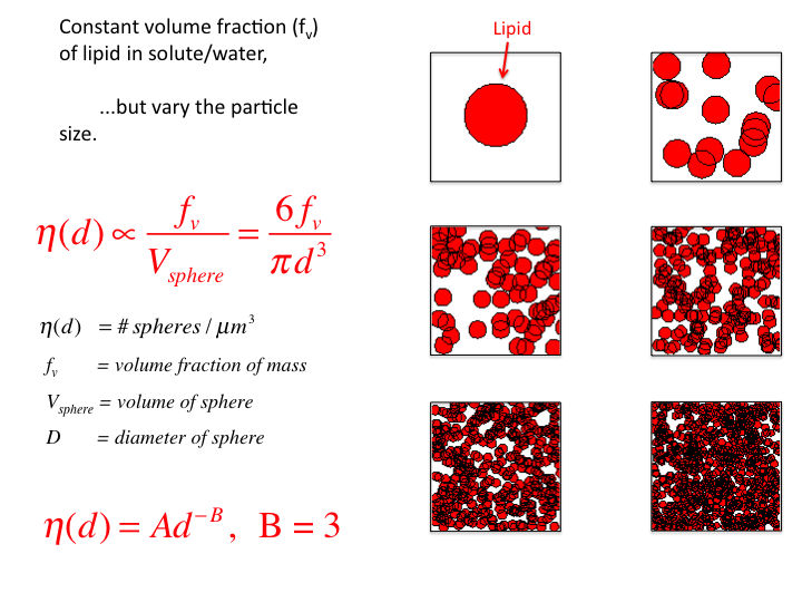
31. Consider a tissue with a volume fraction of lipid fv =
0.10 (n = 1.46, within a salty proteinaceous medium of n = 1.35). Let
the diameter (d) of the droplets vary while keeping the fv
constant. As the size decreases, the number density increases to keep
fv constant. Consequently, the size distribution η(d)
varies as d-3, and B = 3.
slide 32
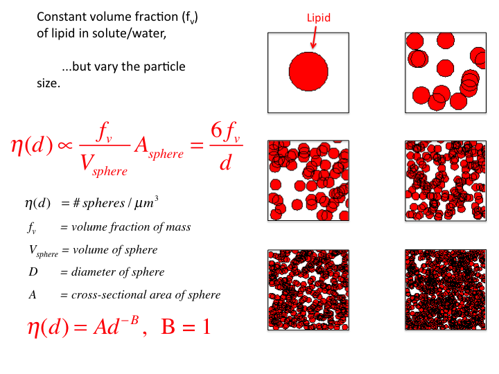
32. If one scales this η(d) by the cross-sectional area of the
spheres, Asphere, then the η(d) varies as d-1,
and B = 1. This scaling is not justified by any physical rationale, but
simply shows what is required to cause η(d) to vary as
d-1.
slide 33
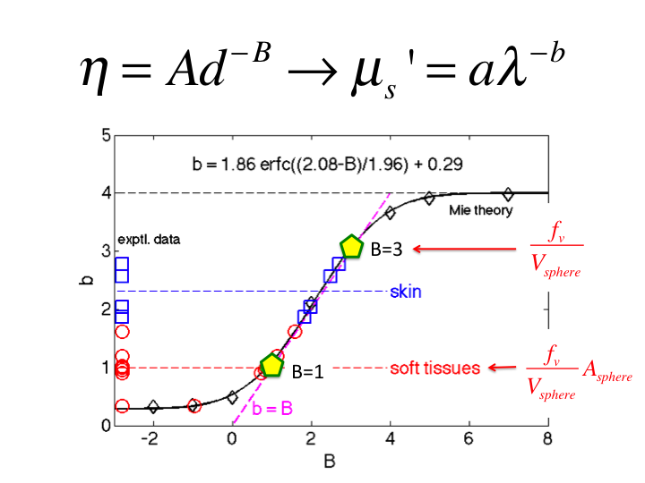
33. Hence, the behavior of tissue falls between these to descriptions of
η(d), scaling as d-3 and d-1.
slide 34
34. The alternative description of light scattering is the continuum
model for light scattering. This paper by Xu and Alfano (2005) was an
early paper on this topic, and utilized the data from Schmitt and Kumar
(1996) that described the distribution of spatial frequencies of
density fluctuation in tissues. I will not attempt to summarize the
continuum model, but I do note that it eventually predicts the
aλ-b behavior of light scattering in tissues. Hence,
both the Mie Theory and Continuum Theory eventually find their
justification in matching experimental data.
slide 35
35. Schmitt and Kumar specified the distribution of spatial frequencies
in several tissues (figure shows liver).
slide 36
36. Xu and Alfano mapped the distribution of spatial frequencies into an
aλ-b behavior of light scattering in tissues.
slide 37
37. A recent paper by Xu et al. (J Biomedical Optics 2008) is especially
informative. It reports on the angular dependence of scattering, as
compared to the Mie Theory prediction of scattering from a cell and a
nucleus, and the Continuum Theory prediction of scattering from the
sub-cellular nanoarchitecture, which dominates the scatter at angles
broader than 20 degrees.
slide 38
38. The relative contributions to scatter from the bare cell, the
nucleus and the nanoarchitecture are shown as a function of angle. Above
20 degrees the nanoarchitecture dominates the scattering.
slide 39
39. A variety of measurements of optical scattering by tissues is
possible. One example is confocal reflectance microscopy, which involves
delivery and collection of light from a confocal volume of tissue.
slide 40
40. A study by the group at Dartmouth College used a confocal
reflectance spectrometer to yield reflectance versus wavelength, R =
aλ-b. This is approximately similar to the story of
µs' = aλ-b. A colon polyp is pressed
against glass and an image taken, which does not show much structure.
However, the image achieved by scanning the confocal spectrometer
yielded an image based on b, which shows a lot of structure in the
polyp. Hence, the scattering power b serves as a contrast parameter for
imaging.
Summary
In summary, optical measurements that
measure the scattering coefficient, µs, and the
anisotropy of scattering, g, can characterize the effective size
distribution of the nanoarchitecture of tissues, as well as the
contributions from the bare cell and the nucleus. Hence, non-invasive
optical measurements can monitor ultrastructure changes in cells and
tissues.