Monte Carlo
simulations of light transport
in turbid
media.
https://omlc.org/classroom/ece580CLT/mc/class1/howtomcsub/index.html
Steven L. Jacques
January, 2002
Table of Contents
1. Introduction
2. The program mcmain.c
2.1 Header
2.2 main()
2.3 Call mcsub()
2.4 Save files
3.
The subroutines
3.1 mcsub()
3.2 Rfresnel()
3.3 SaveFiles()
3.4 RandomNumber()
3.5 Memory allocation routines
4.
Listing of mcmain.c
1. Introduction
This chapter presents a Monte Carlo program written in ANSI Standard C that simulates the penetration of light into a light-scattering medium such as biological tissue.
The program uses a simple steady-state Monte Carlo subroutine, mcsub(),that launches photons as either (1) a collimated beam of variable beam radius, (2) a focused Gaussian beam with variable beam radius, focal depth, and focal waist radius, or (3) an isotropic point source at a chosen depth. The results returned by the subroutine are the concentration of light within the tissue and the escaping light at the tissue surface.
The concentration of light within the tissue is reported as the “fluence rate” F(z,r) in units of [W/cm2] per W of incident power, which equals the energy density of light in a local volume, [J/cm3], times the speed of light, [cm/s]. The escaping light is reported as the “flux density” J(r) in units of [W/cm2] per W of incident power, which equals the power per unit surface area escaping the medium across a local area of the air/medium surface. The parameters z and r indicate depth and radial position [cm], respectively.
The program mcmain() uses the subroutine mcsub()to execute the Monte Carlo simulation. The mcsub() is a concise implementation of the Monte Carlo method. The subroutine utilizes several other subroutines which are also listed within mcmain() and explained later.
The history of this Monte Carlo simulation began with a simple Monte Carlo simulation written by the author that implemented the Henyey-Greenstein scattering function and a mismatched air/tissue boundary. The program was improved by incorporating the step size selection based on a random number as used by Wilson and Adam 1983 [[1]] who first applied a Monte Carlo method to light transport in biological tissues using isotropic scattering. Keijzer et al. 1989 [[2]] improved on the tracking of photon trajectories during simulations of transport in tissue. Keijzer et al. 1989 [[3]]applied Monte Carlo to tissue autofluorescence. Drawing from the work of Witt 1977 [[4]] who provided the basics of Monte Carlo modeling, Prahl et al. 1989 [[5]]translated Keijzer’s work from cylindrical coordinates to Cartesian coordinates that yielded simpler code, and and implemented the selection of deflection angles using random numbers for Henyey-Greenstein scattering. Wang et al. (1992) [[6]] and (1995) [[7]]converted Prahl’s work into modularized ANSI Standard C code for multilayered tissues called MCML which has been widely promulgated. Jacques (1998) [[8]] reduced the MCML code to its simplest form, called mc321.c, to provide a simple simulation of light propagation from point, line, and planar sources of light. For this chapter, the mc321.c code was converted to a subroutine called mcsub() that provides for three dimensional photon propagation from a collimated beam, a focused Gaussian beam, or an isotropic point source with a surface boundary with mismatch refractive indices such as an air/tissue surface.
In summary, this chapter illustrates the use of the Monte Carlo method to model the transport of light within a light-scattering light-absorbing tissue. A listing of mcmain.c with all the required subroutines is provided.
2.
The program mcmain.c
The overall organization of the program mcmain.c is shown below. Each part is discussed in more detail in the following sections. The main() routine within mcmain.c calls a Monte Carlo subroutine, mcsub() that encapsulates the basic Monte Carlo algorithm. The program mcmain.c sets up the desired simulation parameters and calls mcsub() to execute the desired Monte Carlo simulation.
/* mcmain.c
*/
header
declare
subroutines
main() {
Set up variables and arrays.
Call Monte
Carlo subroutine.
Save
escaping flux Jx(r) and fluence rate distribution Fx(z,r).
}
list
subroutines
2.1
Header
The initial header portion of mcmain.c sets up the main() program. The initial #include commands incorporate supporting standard C program files that are needed by the program. The #define commands cause global substitutions of the first argument by the second argument, i.e. USERLABEL is replaced by the string “an example Monte Carlo simulation” and BINS is replaced by the value 101. Thus the user can conveniently change the number of bins used by arrays in the program, and can specify a label that prints out during the run.
The subroutine declarations inform main() of the availability of subroutines listed at the end of the mcmain.c:
mcsub() executes a modular Monte Carlo simulation,
RFresnel() evaluates the value of internal reflectance at the tissue/air surface,
SaveFile() saves the escaping flux density J(r) and fluence rate F(z,r) to a file,
RandomGen() is the random number generator,
and four subroutines for allocation of memory:
nrerror() used if error encountered during memory
allocation,
*AllocVector() allocates memory for a 1-D array,
**AllocMatrix() allocates memory for a 2-D array,
FreeVector() frees the memory allocated for a 1-D array,
FreeMatrix() frees the memory allocated for a 2-D array.
2.2 main()
The main() program organizes the user’s problem, calls the modular subroutine mcsub(), interprets the results, and saves the results to files.
The main() program begins with declarations of the variables used in main(). The first set of variables are USER CHOICES where the user can specify the optical properties of the medium at a particular wavelength.
The parameter mcflag determines whether photons will be launched as a collimated flat-field beam (mcflag = 0), as an approximation to a focused Gaussian beam (mcflag = 1), or as an isotropic point source (mcflag ≥ 2). For flat or Gaussian beams, the parameter radius determines the radius of the beam incident at the surface. In the case of the focused Gaussian beam, radius is the 1/e point radius of the beam at the surface of the medium. For the focused Gaussian beam, an additional pair of parameters describes the focus point under conditions of matched boundary conditions. The parameter waist is the 1/e radius of the Gaussian beam at the focal point, and the parameter zfocus is the depth position of the focal point, both for a matched boundary condition. However, when a Gaussian beam is launched into a tissue with a mismatched boundary condition, mcsub() will calculate the specular reflectance and the refraction of the beam at the external medium/internal medium interface. The parameters xs, ys, zs are used when mcflag ≥ 2 to describe the position of isotropic launching. When mcflag equals 0, 1 or 2, the subroutine mcsub() will printout progress reports to the user during the Monte Carlo simulation. If mcflag > 2, then mcsub() will behave as if mcflag = 2 but will omit any printouts. The number of photons to be launched by mcsub() is set by Nphotons. In summary,
mcflag Radius waist
zfocus xs ys zs
Collimated 0
+ - - - - -
Focused Gaussian 1
+ + + - - -
Isotropic point ≥2
- - - + + +
where + means “uses” and – means “ignores.”
The user chooses the number of photons to be launched by mcsub() by specifying the parameter Nphotons.
The user also chooses the size of the bins for depth, dz, and radial position, dr, appropriate for the cylindrical coordinates used to record escaping flux density J(r) and fluence rate F(z,r). The values (BINS-1)*dz and (BINS-1)*dr specify the total depth and radial extent over which results are stored. The last bins, iz = BINS and ir = BINS, are used to collect any overflow consisting of photons that migrate beyond the extet of the bins.
The remaining variables are determined by the program and the user need not specify their values. All units are in [cm] or variations such as [cm-1] or [cm2]. The declaration and memory allocation of the 1D array (Jx) and the 2D array (Fx) employ memory allocation subroutines described in section 6.5.
There is a printout of the USER CHOICES so that the user can be reminded of the conditions of a simulation when reviewing a printout. A final initialization step sets all to arrays to zero. The indices [iz][ir] specify the particular z and r bins, respectively.
2.3 Call mcsub()
The first part of program considers the penetration of excitation light into the tissue or medium. The control parameters for the Monte Carlo subroutine to be used for the excitation were already set in the USER CHOICES section above. The mcsub() routine is called. The arguments of the subroutine include the optical properties of the medium at the excitation wavelength (muax, musx, gx, n1, n2), the number of r and z bins and their bin sizes and the number of photons to be launched (NR, NZ, dr, dz, Nphotons), the control parameters (mcflag, xs, ys, zs, radius, waist, zfocus), and the array pointers Jx[] and Fx[][] which will hold the results for escaping flux density Jx(r) [W/cm2/W] and fluence rate Fx(z,r) [W/cm2/W]. The subroutine mcsub() records its results in cylindrically symmetric radial coordinates of z and r. The results have been normalized by Nphotons so the same answer is obtained regardless of the value of Nphotons used, although for a low choice of Nphotons the results are more noisy.
2.4 Save files
Finally, the flux density Jx[ir] and fluence rate Fx[iz][ir] are sent to the subroutine SaveFile() that saves the data along with the appropriate r and z positions of each bin based on the function arguments (NR, NZ, dr, dz). The parameter mcflag is also an argument of SaveFile() and specifies the name of the files to be saved. For the case of mcflag = 0 the saved files are called “J0.dat” and “F0.dat”, for the case of mcflag = 1 the saved files are called “J1.dat” and “F1.dat”, and so forth.
3. The subroutines
3.1 mcsub()
The Monte Carlo simulation is executed using a subroutine called mcsub() that considers a semi-infinite medium with an upper surface boundary. The subroutine has the arguments:
mua absorption coefficient
mus scattering coefficient
g anisotropy of scattering
n1 refractive index of internal medium
n2 refractive index of external medium
NR number of r bins
NZ number of z bins
dr incremental size of r bins
dz incremental size of r bins
Nphotons number of photons to be launched
mcflag control of the launch as collimated, focused, or isotropic
xs, ys, zs location of isotropic launching
radius radius of collimated beam or 1/e radius of focused Gaussian beam
waist radius of Gaussian beam at the focal point
zfocus depth position of the focal point for Gaussian beam
*J pointer to 1D array of flux density escaping at surface, J[ir]
**F pointer to 2D array of fluence rate, F[iz][ir]
The subroutine follows an algorithm that is depicted in Figure 1. The program begins with SETUP, declaring and initializing the various variables. In particular, J[ir] and F[iz][ir] are set initially to values of zero.
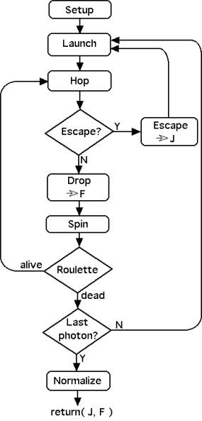
Figure 1: Algorithm for the Monte Carlo subroutine mcsub().
The LAUNCH do-loop proceeds to launch the requested number of photons, Nphotons. If a photon escapes at the surface or is terminated by the ROULETTE procedure, then a new photon is launched. Each photon launching sets the initial photon weight W to a value 1.0 - rsp where rsp is the specular reflectance at the air/tissue surface. The escaping flux density J[ir] returned by mcsub() does not include rsp. The photon launching is executed as either a collimated beam (mcflag = 0), a focused Gaussian beam (mcflag = 1), or an isotropic point source (mcflag ≥ 2).
For a collimated beam, the radial position r of launch is selected based on a random number, rnd, and is assigned to the coordinate x while y and z are assigned the value 0:
x = radius*sqrt(rnd);
y = 0;
z = 0;
where radius is the beam radius provided as an argument of mcsub(). The photon trajectory is specified by the cosine of the angle of the trajectory relative to each of the x, y, and z axes, and these cosine(angle) values are called ux, uy, and uz, respectively. A collimated beam would have uz equal to 1 while ux and uy are assigned the value 0:
ux = 0;
uy = 0;
uz = 1;
The value of the specular reflectance, rsp, is calculated based on the refractive indices n1 and n2:
![]()
For a focused Gaussian beam, the radial position of launch is determined:
x = radius*sqrt(-log(rnd));
y = 0;
z = 0;
where radius is the 1/e radius of the Gaussian beam at the tissue surface. Note that log() is a base e logarithm function. The focus of the Gaussian beam for a matched boundary condition is specifed by zfocus and broadness of the focus is specified waist which is the 1/e radius of the beam at zfocus. The ratio waist/radius is used to scale the launch position x at the surface to yield a radial position xfocus at the depth zfocus, and the trajectory is oriented inward toward the central axis pointing to the position (xfocus,0,zfocus):
xfocus = x*waist/radius;
The program then computes the trajectory required for launching at the surface at position (x,0,0) toward the focus at position (xfocus,0,zfocus), characterized by ux,uy,uz. This trajectory is for the case of matched boundary conditions.
temp = sqrt((x -
xfocus)*(x - xfocus) + zfocus*zfocus);
sintheta = -(x -
xfocus)/temp
costheta = zfocus/temp;
ux = sintheta;
uy = 0.0;
uz = costheta;
This incident trajectory is then modified if there is a mismatched boundary condition. The refractive indices of the internal medium (the tissue), n1, and the external medium (the air), n2, determine the amount of specular reflectance that occurs upon entry into the tissue and the refraction that changes the photon trajectory. The subroutine RFresnel()determines the rsp for the angle of launch that is selected. The angle of transmission is returned as the variable uz.
rsp = RFresnel(n2, n1,
costheta, &uz);
sintheta = sqrt(1.0 -
uz*uz);
ux = -sintheta;
uy = 0.0;
uz = costheta;
Each photon is launched at a different angle and experiences a different rsp. The refraction at the mismatched boundary where n1 > n2 causes the focal point to move deeper into the tissue. Figure 2 illustrates the launching of a Gaussian beam that would focus at zfocus = 0.0300 cm under matched boundary.
Figure 2: Illustration of launching photons as a focused Gaussian beam. Example has radius = 0.0300 cm, waist = 0.0030 cm, zfocus = 0.0300 cm, and matched boundary conditions. Ten launching trajectories are shown as lines.
For an isotropic point source, the position of launch is specified by xs, ys, zs in the argument for mcsub(). The trajectory is isotropic and so has no preferential direction, and is specified:
costheta = 1.0 - 2.0*RandomGen(1,0,NULL);
sintheta = sqrt(1.0 -
costheta*costheta);
psi =
2.0*PI*RandomGen(1,0,NULL);
cospsi = cos(psi);
if (psi < PI)
sinpsi = sqrt(1.0 - cospsi*cospsi);
else
sinpsi = -sqrt(1.0 - cospsi*cospsi);
ux = sintheta*cospsi;
uy = sintheta*sinpsi;
uz = costheta;
The value sin(psi) is calculated as sinpsi = sqrt(1.0 - cospsi*cospsi) since the sqrt() function is faster than the sin() function. Because the launch point is within the tissue, there is no specular reflectance and rsp is set equal to zero.
For each photon launched, the specular reflectance rsp is calculated by one of the three methods above. Then the initial weight of that photon is set to 1.0 – rsp. Hence, a total weight of W = 1.0 is delivered to the tissue but only 1.0 - rsp actually enters the tissue. The resulting J[] therefore does not include specular reflectance. The photon’s status is initiated as photon_status = ALIVE where ALIVE has a Boolean value of 1.
Once a photon is launched, it enters the PROPAGATION CYCLE. The HOP section sets the stepsize s of that the photon takes and updates the current photon position (x,y,z) based on the current trajectory (ux,uy,uz):
s = -log(rnd)/mut;
x += s*ux;
y += s*uy;
z += s*uz;
The
ESCAPE? step asks if (z
<= 0) and if yes then the
photon is attempting to escape out the top surface of the medium. Then the ESCAPE section checks for
total internal reflectance by calling a random number rnd and asking
if (rnd >
RFresnel(n1, n2, -uz, &uz1))
If
yes, then the photon has escaped the tissue and its weight W
is added to the current escaping flux J[ir]. The ESCAPE section resets the photon
position then takes a partial step size to just reach the surface. The radial
position r is calculated based on the x and y
positions and the choice of ir is made by the equivalent of an absolute
value function, ir =
(long)(r/dr) + 1, with the
minimum value being 1 to indicate the first bin. Then the photon is terminated
by setting photon_status =
DEAD, where DEAD has a Boolean value of 0. The photon will bypass the
following DROP-SPIN-ROULETTE section and reaches the end of the PROPAGATION
CYCLE. Because the photon_status =
DEAD a new photon is
launched.
If no, then the photon does not escape
but is internally reflected, accomplished by setting z = -z. The photon_status remains ALIVE so
the photon can enter the DROP-SPIN-ROULETTE section. The DROP section causes the current weight W to decrement by
an amount that depends on the albedo = mus/(mua + mus):
absorb = W*(1 -
albedo);
W -= absorb;
Then
the value absorb is added to the current bin F[iz][ir]. The SPIN
section causes the trajectory of the photon to deviate by an angle theta
specified as costheta = cos(theta) based on sampling the
Henyey-Greenstein scattering function using a random number rnd:
temp = (1.0 - g*g)/(1.0
- g + 2*g*rnd);
costheta = (1.0 + g*g -
temp*temp)/(2.0*g);
Also,
an azimuthal angle psi for the trajectory change is chosen:
psi =
2.0*PI*RandomGen(1,0,NULL);
These
angles of deviation are used to calculate a new trajectory assigned to (ux,uy,uz).
The
ROULETTE section provides a means of terminating a photon based on
absorption. A value THRESHOLD was set equal to 1e-4 at the beginning of the subroutine.
If the weight W drops below THRESHOLD, then the photon is either terminated or
its weight W is increased and propagation continues. A random number rnd is
obtained and compared with a value CHANCE set to
0.1 in this program. The program asks if rnd < CHANCE,
and if yes then the weight is increased by a factor 1/CHANCE or 10-fold. Propagation continues and the photon returns to
the top of the PROPAGATION CYCLE.
If no, then the photon is terminated by setting photon_status = DEAD. At the end of the PROPAGATION CYCLE a
new photon is launched. This method statistically conserves photon energy but
allows for a means to terminate photons.
After
the PROPAGATION CYCLE has launched Nphotons, the
simulation is complete. The
subroutine now normalizes the values in J[ir] by the
area of the [ir] bins to yield the escaping flux density
[W/cm2/W]. The
subroutine normalizes the values in F[iz][ir] by the
bin volumes to yield the density of power deposition [W/cm3/W].
Further normalization by the absorption coefficient mua
[cm-1] yields the fluence rate [W/cm2/W]. The subroutine
returns J[] and F[][] to
the calling program mcmain().
To
test mcsub(), an example problem was run which could
be compared with diffusion theory. The optical properties were mua
= 1 cm-1, mus = 100 cm-1, g
= 0.90. The refractive indices of the internal and external media were 1.33 and
1.00, respectively, simulating a water/air interface. An isotropic point source
was launched at a depth of zs
= 1/(mua + mus*(1‑g))
or 0.09091 cm.
Figure
3 shows the comparison of the mcsub() result
and diffusion theory as outlined by Farrel et al. (1992) [[9]]
using the extrapolated boundary condition:
![]()
where
where
ri is the total internal reflectance at the tissue surface. The
difference between Monte Carlo and diffusion theory is characterized by the
ratio (DT – MC)/MC where DT is the J(r) calculated by diffusion theory
and MC is the J(r) calculated by mcsub(). The
ratio is in the range of –0.20 to 0.10, except near r = 0 where DT is far
too low. This is basically the same behavior predicted by the MCML code [6].
Figure 3: Testing mcsub() versus diffusion theory.
(TOP) Escaping flux density J(r) versus radial position r. (BOTTOM) Ratio (DT
– MC)/MC where DT is J(r) calculated by diffusion theory and MC is J(r)
calculated by mcsub().
Optical properties: ma = 1
cm–1, ms =1
00 cm–1, g = 0.90, n1 = 1.33, n2 = 1.00.
Isotropic point source at 1 mean free path below surface, i.e. zs = 1/(ma + ms(1-g)).
Another
test was to compute the total escaping flux, Jtot [W/W],
![]()
for
the optical properties: ma = 1 cm-1, ms
= 9 cm-1, g = 0.0, yielding an albedo = 0.90. The medium was
semi-infinite and the surface boundary condition was matched. This problem has
been simulated by Prahl (1988) [[10]]
who reported in his Table 3-1 the result to be 0.4149 and that this value
matched the published value of van de Hulst (1980) [[11]]. The mcsub()
was run ten times with ten different Seed values to
yield a mean and standard deviation of 0.41507 ± 0.00018 (n = 10).
3.2 RFresnel()
The subroutine RFresnel() was prepared by Lihong Wang as part of the MCML code [6]. The subroutine computes the Fresnel reflectance at an interface between two media with refractive indices ni and nt where ni is the medium from which the incident photon arrives and nt is the medium into which the photon transmits. The angle of incidence is specifed as ca1 = cos(angle of incidence). The angle of transmission is calculated based on Snell’s Law by the subroutine and the cos(angle of transmission) is returned as the value of the variable ca2_Ptr:
RFresnel(ni, nt, ca1,
*ca2_Ptr)
During photon launch as a focused Gaussian beam, the incident medium refractive index is assigned the value of the external medium (ni = n2) and the transmitted medium refractive index is assigned the value of the internal medium (nt = n1). The specular reflectance rsp and the cos(angle of transmission), uz, are calculated by the subroutine call:
rsp = RFresnel(n2, n1,
costheta, &uz);
During photon propagation as photons attempt to escape the medium, they are tested for the occurence of total internal reflectance. In this case, the incident medium refractive index is the value of the internal medium (ni = n1) and the transmitted medium refractive index is assigned the value of the external medium (nt = n2). The incident cos(angle) is the negative of the current value uz which is negative because the photon is escaping, so -uz is positive. The transmitted angle uz1 is not used, but does specify the cos(angle of transmission) for the escaping photon and could be used to document the angle of escape. The test for photon escape is phrased:
if (rnd >
RFresnel(n1, n2, -uz, &uz1))
and if true then there is escape and if false then there is total internal reflectance.
3.3 SaveFiles()
The SaveFiles() subroutine saves two files, J[ir] and F[iz][ir], along with the appropriate values of r[ir] and z[iz]. The names of the files depends on the values of the argument Nfile:
SaveFile(*J, **F,
Nfile, NR, NZ, dr, dz)
where NR and NZ are the number of bins and dr and dz are the incremental bin sizes. If Nfile equals 1, then the names of the files are J1.dat and F1.dat. If Nfile equals 2, then the names of the files are J2.dat and F2.dat, and so on.
The values of r[ir] and z[ir] are calculated:
r[ir] = (ir –
0.5)*dr
z[iz] = (iz –
0.5)*dz
which are the midpoints of each bin. The calculation for r[ir] is based on the expectation value for r within the [ir] bin, assuming that the general form of the J[ir] and F[iz][ir] responses versus r is 1/r. Then the expectation value is:
which is the midpoint of the [ir] bin. A more correct assignment of r[ir] would involve using the true behavior of J and F versus r, but this leads to iteratively reconsidering an assignment after an initial determination of the behavior. The user is better advised to simply run the mcsub() with smaller values of dr and dz if the user wishes to refine the estimate of behavior J and F at small r.
The file J.dat is a file with two columns and NR rows. The first column is r[ir]. The second column is J[ir]. The file F.dat is a file with NR+1 columns and NZ+1 rows. The first element (1,1) is ignored, and is set equal to 0. The first column, rows 2 to NZ+1, lists the values of z[iz]. The first row, columns 2 to NR+1, lists the values of r[ir]. The remaining array, rows 2 to NZ+1, columns 2 to NR+1, holds the values of F[iz][ir].
3.4 RandomNumber()
The random number generator subroutine was prepared by Lihong Wang as part of the MCML code [6]:
RandomGen(Type, Seed, *Status)
The generator is initialized by the call with Type set to 0 and Seed set to a long integer (0 < Seed < 32000), for example set equal to 1:
RandomGen(0,1,NULL);
Subsequently, a random number rnd is generated by the call with Type set to 1:
rnd =
RandomGen(1,0,NULL);
In some cases, such as when the a command must evaluate log(rnd), it is important to exclude the value rnd = 0. In such cases, the call is phrased:
while ((rnd =
RandomGen(1,0,NULL)) <= 0.0);
3.5 Memory allocation routines
The memory allocation routines were also prepared by Lihong Wang as part of the MCML code [6]. The routines are
nrerror(error_text[]);
*AllocVector(nl, nh);
**AllocMatrix(nrl, nrh,
ncl, nch);
FreeVector(*v, nl, nh);
FreeMatrix(**m, nrl,
nrh, ncl, nch);
They are used in declaring 1D and 2D arrays at the beginning of the program mcmain() and in freeing the memory allocated for these arrays at the end of mcmain(). They allow the arrays to be addressed by indices ranging from 1 to NR and 1 to NZ. Their use is shown in mcmain().
4. Listing of mcmain.c
/*************
* mcmain.c
*************/
#include <stdio.h>
#include <stdlib.h>
#include <string.h>
#include <math.h>
#include <time.h>
/*************************/
/**** USER CHOICES ******/
/*************************/
#define USER_LABEL
"mcmain.c for class"
#define BINS 101
/*************************/
/*************************/
/**********************
* DECLARE SUBROUTINES
*********************/
/* The Monte Carlo subroutine */
void mcsub(double mua, double mus, double g, double n1, double n2,
long
NR, long NZ, double dr, double dz, double Nphotons,
int
mcflag, double xs, double ys, double zs,
double
radius, double waist, double zfocus,
double
*J, double **F);
/* Computes internal reflectance at tissue/air interface */
double RFresnel(double n1, double n2, double ca1, double *ca2_Ptr);
/* Saves surface escape R(r) and fluence rate distribution F(z,r)
*/
void SaveFile(double *J, double **F, int Nfile,
long NR, long NZ, double dr, double dz);
/* Random number generator
Initiate by
RandomGen(0,1,NULL)
Use as rnd =
RandomGen(1,0,NULL) */
double RandomGen(char Type, long Seed, long *Status);
/* Memory allocation routines
* from MCML ver. 1.0,
1992 L. V. Wang, S. L. Jacques,
* which are modified
versions from Numerical Recipes in C. */
void
nrerror(char error_text[]);
double *AllocVector(short nl, short nh);
double **AllocMatrix(short nrl,short nrh,short ncl,short nch);
void
FreeVector(double *v,short nl,short nh);
void
FreeMatrix(double **m,short nrl,short nrh,short ncl,short nch);
/**********************
* MAIN PROGRAM
*********************/
int main() {
/**** Declare variables ******/
double mua; /* excitation absorption coeff.
[cm^-1] */
double mus; /* excitation scattering coeff.
[cm^-1] */
double g; /* excitation
anisotropy [dimensionless] */
double n1; /* refractive index of
medium */
double n2; /* refractive index outside
medium */
short
mcflag; /* 0 = collimated, 1 = focused Gaussian,
2 = isotropic pt */
double radius;
/* used if mcflag = 0 or 1 */
double
waist; /* used if mcflag =
1 */
double zfocus;
/* used if mcflag = 1 */
double xs; /* used if mcflag = 2
*/
double ys; /* used if mcflag = 2
*/
double zs; /* used if mcflag = 2
*/
/* other parameters */
double
Nruns; /* number photons
launched = Nruns x 1e6 */
double dr; /* radial bin size
[cm] */
double dz; /* depth bin size
[cm] */
char
label[1];
double Nphotons;
long
ir, iz;
double temp; /*
dummy variables */
double
start_time, finish_time1; /* for clock() */
double timeA,
timeB;
time_t now;
double *Jx;
double **Fx;
long
NR = BINS; /* number of radial bins */
long
NZ = BINS; /* number of depth bins */
Jx = AllocVector(1,BINS);
Fx = AllocMatrix(1, BINS, 1,
BINS); /* for absorbed excitation */
strcpy(label, USER_LABEL);
printf("\n||-------------------------\n");
printf( "||
%s\n",label);
printf(
"||-------------------------\n\n");
start_time = clock();
now = time(NULL);
printf("%s\n", ctime(&now));
/*************************/
/**** USER CHOICES ******/
/*************************/
mua =
1.0; /* excitation absorption
coeff. [cm^-1] */
mus =
100.0;/* excitation scattering coeff. [cm^-1] */
g
= 0.90; /* excitation anisotropy [dimensionless] */
n1 =
1.33; /* refractive index of medium */
n2 =
1.00; /* refractive index outside medium */
mcflag = 0;
/* 0 = collimated, 1 = focused Gaussian,
2 = isotropic pt */
radius = 0.0; /* used
if mcflag = 0 or 1 */
waist = 0.0; /* used if mcflag = 1 */
zfocus = 0.0; /* used
if mcflag = 1 */
xs =
0.0; /* used if mcflag = 2 */
ys =
0.0; /* used if mcflag = 2 */
zs =
0.090909; /* used if mcflag = 2 */
/* other parameters */
Nruns = 0.01; /* number photons launched
= Nruns x 1e6 */
dr =
0.0100; /* radial bin size [cm] */
dz =
0.0100; /* depth bin size [cm] */
if (1) { /* Switch printout ON=1 or OFF=0 */
/*
print out summary of parameters to user */
printf("-----
USER CHOICES -----\n");
printf("mua = %1.3f\n",mua);
printf("mus = %1.3f\n",mus);
printf("g =
%1.3f\n",g);
printf("n1 = %1.3f\n",n1);
printf("n2 =
%1.3f\n",n2);
printf("mcflag = %d\n" ,mcflag);
printf("radius = %1.4f\n",radius);
printf("waist = %1.4f\n",waist);
printf("zfocus = %1.4f\n",radius);
printf("xs =
%1.4f\n",xs);
printf("ys =
%1.4f\n",ys);
printf("zs =
%1.4f\n",zs);
printf("OTHER\n");
printf("Nruns = %1.1e\n",Nruns);
printf("dr =
%1.4e\n",dr);
printf("dz =
%1.4e\n",dz);
printf("---------------\n\n");
}
/* Initialize arrays */
for (ir=1; ir<=NR; ir++) {
Jx[ir]
= 0.0;
for
(iz=1; iz<=NR; iz++) {
Fx[iz][ir]
= 0.0;
}
}
/* Time completion estimate */
timeA = clock();
mcsub( mua,
mus, g, n1, n2, /* CALL THE
MONTE CARLO SUBROUTINE */
NR,
NZ, dr, dz, 1000,
mcflag,
xs, ys, zs,
radius,
waist, zfocus,
Jx,
Fx);
/* returns J, F */
timeB = clock();
temp = (timeB - timeA)/CLOCKS_PER_SEC/60/1000; /* min per photon */
printf("%5.3e min/photon \n", temp);
printf("estimated completion times = %5.2f min\n",
temp*1e6*Nruns);
/*********************
* CALL mcsub()
*********************/
Nphotons = 1e6*Nruns;
mcsub( mua,
mus, g, n1, n2, /* CALL THE
MONTE CARLO SUBROUTINE */
NR,
NZ, dr, dz, Nphotons,
mcflag,
xs, ys, zs,
radius,
waist, zfocus,
Jx,
Fx);
/* returns J, F */
/* Save results to files Ji.dat and Fi.dat, where i = mcflag. */
SaveFile(Jx, Fx, mcflag, NR, NZ, dr, dz);
printf("------------------------------------------------------\n");
finish_time1 = clock();
printf("-------------------------------------------------------------\n");
printf("Elapsed Time for excitation = %5.2f min\n",
(double)(finish_time1-start_time)/CLOCKS_PER_SEC/60);
now = time(NULL);
printf("%s\n", ctime(&now));
FreeVector(Jx, 1, BINS);
FreeMatrix(Fx, 1, BINS, 1, BINS);
return(0);
}
/**********************************************************
*
SUBROUTINES
**********************************************************/
/**********************************************************
* The Monte Carlo
SUBROUTINE
**********************************************************/
void mcsub(double mua, double mus, double g, double n1, double n2,
long
NR, long NZ, double dr, double dz, double Nphotons,
int
mcflag, double xs, double ys, double zs,
double
radius, double waist, double zfocus,
double
*J, double **F)
{
/* Constants */
double PI = 3.1415926;
short ALIVE = 1; /* if
photon not yet terminated */
short DEAD =
0; /* if
photon is to be terminated */
double THRESHOLD = 0.0001; /*
used in roulette */
double CHANCE = 0.1; /*
used in roulette */
/* Variable parameters */
double mut,
albedo, absorb, rsp, Rsptot, Atot;
double rnd,
xfocus;
double x,y,z,
ux,uy,uz,uz1, uxx,uyy,uzz, s,r,W,temp;
double psi,costheta,sintheta,cospsi,sinpsi;
long iphoton, ir, iz, CNT;
short photon_status;
/**** INITIALIZATIONS *****/
RandomGen(0,1,NULL); /* initiate with seed = 1, or any long
integer. */
CNT = 0;
mut = mua
+ mus;
albedo = mus/mut;
Rsptot = 0.0; /* accumulate absorbed photon weight */
Atot = 0.0; /*
accumulate specular reflectance per photon */
/* initialize arrays to zero */
for (ir=1; ir<=NR; ir++) {
J[ir]
= 0.0;
for
(iz=1; iz<=NZ; iz++)
F[iz][ir]
= 0.0;
}
/*============================================================
======================= RUN N photons =====================
* Launch N photons,
initializing each one before progation.
============================================================*/
for (iphoton=1; iphoton<=Nphotons; iphoton++) {
/*
Print out progress for user if mcflag < 3 */
temp
= (double)iphoton;
if
((mcflag < 3) & (temp >= 1000)) {
if
(temp<10000) {
if
(fmod(temp,1000)==0)
printf("%1.0f
photons\n",temp);
}
else
if (temp<100000) {
if
(fmod(temp,10000)==0)
printf("%1.0f photons\n",temp);
}
else
if (temp<1000000) {
if
(fmod(temp,100000)==0)
printf("%1.0f photons\n",temp);
}
else
if (temp<10000000) {
if
(fmod(temp,1000000)==0)
printf("%1.0f photons\n",temp);
}
else
if (temp<100000000) {
if
(fmod(temp,10000000)==0)
printf("%1.0f
photons\n",temp);
}
}
/**** LAUNCH
Initialize
photon position and trajectory.
Implements an
isotropic point source.
*****/
if (mcflag == 0) {
/*
UNIFORM COLLIMATED BEAM INCIDENT AT SURFACE */
/*
Launch at (r,z) = (radius*sqrt(rnd), 0).
* Due to cylindrical symmetry, radial
launch position is
* assigned to x while y = 0.
* radius = radius of uniform beam. */
/*
Initial position */
rnd
= RandomGen(1,0,NULL);
x
= radius*sqrt(rnd);
y
= 0;
z
= 0;
/*
Initial trajectory as cosines */
ux
= 0;
uy
= 0;
uz
= 1;
/*
specular reflectance */
temp = n1/n2; /* refractive index
mismatch, internal/external */
temp = (1.0 - temp)/(1.0 + temp);
rsp = temp*temp; /* specular
reflectance at boundary */
}
else if (mcflag == 1) {
/*
GAUSSIAN BEAM AT SURFACE */
/*
Launch at (r,z) = (radius*sqrt(-log(rnd)), 0).
* Due to cylindrical symmetry, radial
launch position is
* assigned to x while y = 0.
* radius = 1/e radius of Gaussian beam
at surface.
* waist = 1/e radius of Gaussian focus.
* zfocus = depth of focal point. */
/*
Initial position */
while
((rnd = RandomGen(1,0,NULL)) <= 0.0); /* avoids rnd = 0 */
x
= radius*sqrt(-log(rnd));
y
= 0.0;
z
= 0.0;
/*
Initial trajectory as cosines */
/*
Due to cylindrical symmetry, radial launch trajectory is
* assigned to ux and uz while uy = 0. */
xfocus
= waist/beam*x;
temp
= sqrt((x - xfocus)*(x - xfocus) + zfocus*zfocus);
sintheta
= -(x - xfocus)/temp;
costheta
= zfocus/temp;
ux
= sintheta;
uy
= 0.0;
uz
= costheta;
/*
specular reflectance and diffraction */
rsp
= RFresnel(n2, n1, costheta, &uz); /* new uz */
ux = -sqrt(1.0 - uz*uz);
/* new ux */
}
else {
/*
ISOTROPIC POINT SOURCE AT POSITION xs,ys,zs */
/*
Initial position */
x
= xs;
y
= ys;
z
= zs;
/*
Initial trajectory as cosines */
costheta
= 1.0 - 2.0*RandomGen(1,0,NULL);
sintheta
= sqrt(1.0 - costheta*costheta);
psi
= 2.0*PI*RandomGen(1,0,NULL);
cospsi
= cos(psi);
if
(psi < PI)
sinpsi
= sqrt(1.0 - cospsi*cospsi);
else
sinpsi
= -sqrt(1.0 - cospsi*cospsi);
ux
= sintheta*cospsi;
uy
= sintheta*sinpsi;
uz
= costheta;
/*
specular reflectance */
rsp
= 0.0;
}
W
= 1.0 - rsp; /* set photon
initial weight */
Rsptot += rsp; /* accumulate
specular reflectance per photon */
photon_status = ALIVE;
/******************************************
****** HOP_ESCAPE_SPINCYCLE **************
* Propagate one photon until it dies by ESCAPE or ROULETTE.
*******************************************/
do {
/**** HOP
* Take step to new
position
* s = stepsize
* ux, uy, uz are
cosines of current photon trajectory
*****/
while
((rnd = RandomGen(1,0,NULL)) <= 0.0); /* avoids rnd = 0 */
s
= -log(rnd)/mut; /* Step
size. Note: log() is base e */
x
+= s*ux; /*
Update positions. */
y
+= s*uy;
z
+= s*uz;
/*
Does photon ESCAPE at surface? ... z <= 0? */
if (z <= 0) {
rnd
= RandomGen(1,0,NULL);
/*
Check Fresnel reflectance at surface boundary */
if
(rnd > RFresnel(n1, n2, -uz, &uz1)) {
/*
Photon escapes at external angle, uz1 = cos(angle) */
x
-= s*ux;
/* return to original position */
y
-= s*uy;
z
-= s*uz;
s = fabs(z/uz); /* calculate stepsize to
reach surface*/
x
+= s*ux;
/* partial step to reach surface */
y
+= s*uy;
r
= sqrt(x*x + y*y); /* find
radial position r */
ir
= (long)(r/dr) + 1; /* round to 1 <= ir */
if
(ir > NR) ir = NR; /* ir = NR
is overflow bin */
J[ir]
+= W; /*
increment escaping flux */
photon_status
= DEAD;
}
else
z = -z; /* Total internal
reflection. */
}
if (photon_status ==
ALIVE) {
/*********************************************
****** SPINCYCLE = DROP_SPIN_ROULETTE
******
*********************************************/
/****
DROP
* Drop photon weight (W) into local bin.
*****/
absorb
= W*(1 - albedo); /* photon weight
absorbed at this step */
W
-= absorb;
/* decrement WEIGHT by amount absorbed */
Atot
+= absorb; /*
accumulate absorbed photon weight */
/*
deposit power in cylindrical coordinates z,r */
r = sqrt(x*x + y*y); /* current
cylindrical radial position */
ir
= (long)(r/dr) + 1; /* round to 1 <= ir
*/
iz
= (long)(fabs(z)/dz) + 1; /* round
to 1 <= iz */
if
(ir >= NR) ir = NR; /* last bin is for
overflow */
if
(iz >= NZ) iz = NZ; /* last bin is for
overflow */
F[iz][ir]
+= absorb; /* DROP
absorbed weight into bin */
/****
SPIN
* Scatter photon into new trajectory
defined by theta and psi.
* Theta is specified by cos(theta),
which is determined
* based on the Henyey-Greenstein
scattering function.
* Convert theta and psi into cosines ux,
uy, uz.
*****/
/*
Sample for costheta */
rnd
= RandomGen(1,0,NULL);
if
(g == 0.0)
costheta
= 2.0*rnd - 1.0;
else
if (g == 1.0)
costheta
= 1.0;
else
{
temp
= (1.0 - g*g)/(1.0 - g + 2*g*rnd);
costheta
= (1.0 + g*g - temp*temp)/(2.0*g);
}
sintheta
= sqrt(1.0 - costheta*costheta);/*sqrt faster than sin()*/
/*
Sample psi. */
psi
= 2.0*PI*RandomGen(1,0,NULL);
cospsi
= cos(psi);
if
(psi < PI)
sinpsi
= sqrt(1.0 - cospsi*cospsi); /*sqrt faster */
else
sinpsi
= -sqrt(1.0 - cospsi*cospsi);
/*
New trajectory. */
if
(1 - fabs(uz) <= 1.0e-12) { /*
close to perpendicular. */
uxx
= sintheta*cospsi;
uyy
= sintheta*sinpsi;
uzz
= costheta*((uz)>=0 ? 1:-1);
}
else
{ /* usually use this option
*/
temp
= sqrt(1.0 - uz*uz);
uxx
= sintheta*(ux*uz*cospsi - uy*sinpsi)/temp + ux*costheta;
uyy
= sintheta*(uy*uz*cospsi + ux*sinpsi)/temp + uy*costheta;
uzz
= -sintheta*cospsi*temp + uz*costheta;
}
/*
Update trajectory */
ux
= uxx;
uy
= uyy;
uz
= uzz;
/****
CHECK ROULETTE
* If photon weight below THRESHOLD, then
terminate photon using
* Roulette technique. Photon has CHANCE
probability of having its
* weight increased by factor of
1/CHANCE,
* and 1-CHANCE probability of
terminating.
*****/
if
(W < THRESHOLD) {
rnd
= RandomGen(1,0,NULL);
if
(rnd <= CHANCE)
W
/= CHANCE;
else
photon_status = DEAD;
}
}/**********************************************
**** END of SPINCYCLE =
DROP_SPIN_ROULETTE *
**********************************************/
}
while (photon_status == ALIVE);
/******************************************
****** END of
HOP_ESCAPE_SPINCYCLE ******
****** when
photon_status == DEAD) ******
******************************************/
/* If photon dead, then launch new photon. */
} /*======================= End RUN N photons =====================
=====================================================================*/
/************************
* NORMALIZE
* J[ir] escaping flux density [W/cm^2 per W
incident]
*
where bin = 2.0*PI*r[ir]*dr [cm^2].
* F[iz][ir]
fluence rate [W/cm^2 per W incident]
*
where bin = 2.0*PI*r[ir]*dr*dz [cm^3].
************************/
temp = 0.0;
for (ir=1; ir<=NR; ir++) {
r
= (ir - 0.5)*dr;
temp
+= J[ir]; /* accumulate total escaped
photon weight */
J[ir]
/= 2.0*PI*r*dr*Nphotons;
/* flux density */
for
(iz=1; iz<=NZ; iz++)
F[iz][ir]
/= 2.0*PI*r*dr*dz*Nphotons*mua; /* fluence rate */
}
if (mcflag < 2) {
printf("Specular
= %5.6f\n", Rsptot/Nphotons);
printf("Absorbed
= %5.6f\n", Atot/Nphotons);
printf("Escaped = %5.6f\n", temp/Nphotons);
printf("total = %5.6f\n", (Rsptot +
Atot + temp)/Nphotons);
}
} /******** END SUBROUTINE **********/
/***********************************************************
* FRESNEL REFLECTANCE
* Computes reflectance
as photon passes from medium 1 to
* medium 2 with
refractive indices n1,n2. Incident
* angle a1 is
specified by cosine value ca1 = cos(a1).
* Program returns
value of transmitted angle a1 as
* value in *ca2_Ptr =
cos(a2).
****/
double RFresnel(double n1, /* incident refractive index.*/
double
n2, /* transmit
refractive index.*/
double
ca1, /* cosine of the
incident */
/* angle
a1, 0<a1<90 degrees. */
double
*ca2_Ptr) /* pointer to the cosine */
/* of the
transmission */
/* angle
a2, a2>0. */
{
double r;
if(n1==n2) { /** matched boundary. **/
*ca2_Ptr
= ca1;
r
= 0.0;
}
else if(ca1>(1.0 - 1.0e-12)) { /** normal incidence. **/
*ca2_Ptr
= ca1;
r
= (n2-n1)/(n2+n1);
r
*= r;
}
else if(ca1< 1.0e-6)
{ /** very slanted. **/
*ca2_Ptr
= 0.0;
r
= 1.0;
}
else { /**
general. **/
double
sa1, sa2; /* sine of incident and transmission angles. */
double
ca2; /*
cosine of transmission angle. */
sa1
= sqrt(1-ca1*ca1);
sa2
= n1*sa1/n2;
if(sa2>=1.0)
{
/*
double check for total internal reflection. */
*ca2_Ptr
= 0.0;
r
= 1.0;
}
else
{
double
cap, cam; /* cosines of sum ap or
diff am of the two */
/*
angles: ap = a1 + a2, am = a1 - a2. */
double
sap, sam; /* sines. */
*ca2_Ptr
= ca2 = sqrt(1-sa2*sa2);
cap
= ca1*ca2 - sa1*sa2; /* c+ = cc - ss. */
cam
= ca1*ca2 + sa1*sa2; /* c- = cc + ss. */
sap
= sa1*ca2 + ca1*sa2; /* s+ = sc + cs. */
sam
= sa1*ca2 - ca1*sa2; /* s- = sc - cs. */
r
= 0.5*sam*sam*(cam*cam+cap*cap)/(sap*sap*cam*cam);
/*
rearranged for speed. */
}
}
return(r);
} /******** END SUBROUTINE **********/
/***********************************************************
* SAVE RESULTS TO
FILES
* to files named
≥Ji.dat≤ and ≥Fi.dat≤ where i = mcflag.
* Saves
≥Ji.dat≤ in following format:
* Saves r[ir] values in first column, (2:NR,1) = (rows,cols).
* Saves Ji[ir] values in second
column, (2:NR,2) = (rows,cols).
* Saves
≥Fi.dat≤ in following format:
* The upper element (1,1) is filled
with zero, and ignored.
* Saves z[iz] values in first
column, (2:NZ,1) = (rows,cols).
* Saves r[ir] values in first
row, (1,2:NZ) =
(rows,cols).
* Saves Fi[iz][ir] in (2:NZ, 2:NR).
***********************************************************/
void SaveFile( double
*R, double **F, int Nfile,
long
NR, long NZ, double dr, double dz)
{
double r,
z, r1, r2;
long ir, iz;
char name[20];
FILE* target;
/* SAVE flux density J(r) */
sprintf(name, "mcJ%d.dat",Nfile);
target = fopen(name, "w");
for (ir=1; ir<=NR; ir++) {
r2
= ir*dr;
r1
= (ir-1)*dr;
r
= 2.0/3*(r2*r2 + r2*r1 + r1*r1)/(r1 + r2);
fprintf(target,
"%5.5f \t%5.12f\n", r, R[ir]);
}
fclose(target);
/* SAVE fluence rate F(z,r) */
sprintf(name, "mcF%d.dat",Nfile);
target = fopen(name, "w");
fprintf(target, "%5.5f", 0.0); /* ignore upperleft
element of matrix */
for (ir=1; ir<=NR; ir++) {
r2
= ir*dr;
r1
= (ir-1)*dr;
r
= 2.0/3*(r2*r2 + r2*r1 + r1*r1)/(r1 + r2);
fprintf(target,
"\t %5.5f", r);
}
fprintf(target, "\n");
for (iz=1; iz<=NZ; iz++) {
z
= (iz - 0.5)*dz; /* z values for depth position in 1st column */
fprintf(target,
"%5.5f", z);
for
(ir=1; ir<=NR; ir++)
fprintf(target,
"\t %5.12f", F[iz][ir]);
fprintf(target,
"\n");
}
fclose(target);
} /******** END SUBROUTINE **********/
/*********************************************************************
* RANDOM NUMBER
GENERATOR
* A random number
generator that generates uniformly
* distributed
random numbers between 0 and 1 inclusive.
* The algorithm
is based on:
* W.H. Press,
S.A. Teukolsky, W.T. Vetterling, and B.P.
* Flannery,
"Numerical Recipes in C," Cambridge University
* Press, 2nd
edition, (1992).
* and
* D.E. Knuth,
"Seminumerical Algorithms," 2nd edition, vol. 2
* of "The
Art of Computer Programming", Addison-Wesley, (1981).
*
* When Type is 0,
sets Seed as the seed. Make sure 0<Seed<32000.
* When Type is 1,
returns a random number.
* When Type is 2,
gets the status of the generator.
* When Type is 3,
restores the status of the generator.
*
* The status of
the generator is represented by Status[0..56].
* Make sure you
initialize the seed before you get random
* numbers.
****/
#define MBIG 1000000000
#define MSEED 161803398
#define MZ 0
#define FAC 1.0E-9
double RandomGen(char Type, long Seed, long *Status)
{
static long i1, i2, ma[56]; /* ma[0] is not used. */
long mj, mk;
short i, ii;
if (Type == 0) { /* set seed. */
mj
= MSEED - (Seed < 0 ? -Seed : Seed);
mj
%= MBIG;
ma[55]
= mj;
mk
= 1;
for
(i = 1; i <= 54; i++) {
ii
= (21 * i) % 55;
ma[ii]
= mk;
mk
= mj - mk;
if
(mk < MZ)
mk
+= MBIG;
mj = ma[ii];
}
for
(ii = 1; ii <= 4; ii++)
for
(i = 1; i <= 55; i++) {
ma[i]
-= ma[1 + (i + 30) % 55];
if
(ma[i] < MZ)
ma[i]
+= MBIG;
}
i1
= 0;
i2
= 31;
}
else if (Type == 1) { /* get a number. */
if
(++i1 == 56)
i1
= 1;
if
(++i2 == 56)
i2
= 1;
mj
= ma[i1] - ma[i2];
if
(mj < MZ)
mj
+= MBIG;
ma[i1]
= mj;
return
(mj * FAC);
}
else if (Type == 2) { /* get status. */
for
(i = 0; i < 55; i++)
Status[i]
= ma[i + 1];
Status[55]
= i1;
Status[56]
= i2;
}
else if (Type == 3) { /* restore status. */
for
(i = 0; i < 55; i++)
ma[i
+ 1] = Status[i];
i1
= Status[55];
i2
= Status[56];
}
else
puts("Wrong
parameter to RandomGen().");
return (0);
}
#undef MBIG
#undef MSEED
#undef MZ
#undef FAC
/******* end
subroutine ******/
/***********************************************************
* MEMORY ALLOCATION
* REPORT ERROR MESSAGE
to stderr, then exit the program
* with signal 1.
****/
void nrerror(char error_text[])
{
fprintf(stderr,"%s\n",error_text);
fprintf(stderr,"...now exiting to system...\n");
exit(1);
}
/***********************************************************
* MEMORY ALLOCATION
* by Lihong Wang for
MCML version 1.0 code, 1992.
* ALLOCATE A 1D ARRAY with
index from nl to nh inclusive.
* Original matrix and vector
from Numerical Recipes in C
* don't initialize the elements
to zero. This will
* be accomplished by the
following functions.
****/
double *AllocVector(short nl, short nh)
{
double *v;
short i;
v=(double *)malloc((unsigned) (nh-nl+1)*sizeof(double));
if (!v) nrerror("allocation failure in vector()");
v -= nl;
for(i=nl;i<=nh;i++) v[i] = 0.0; /*
init. */
return v;
}
/***********************************************************
* MEMORY ALLOCATION
* ALLOCATE A 2D ARRAY with row
index from nrl to nrh
* inclusive, and column index
from ncl to nch inclusive.
****/
double **AllocMatrix(short nrl,short nrh,
short
ncl,short nch)
{
short i,j;
double **m;
m=(double **) malloc((unsigned) (nrh-nrl+1) *sizeof(double*));
if (!m) nrerror("allocation failure 1 in matrix()");
m
-= nrl;
for(i=nrl;i<=nrh;i++) {
m[i]=(double
*) malloc((unsigned) (nch-ncl+1) *sizeof(double));
if
(!m[i]) nrerror("allocation failure 2 in matrix()");
m[i]
-= ncl;
}
for(i=nrl;i<=nrh;i++)
for(j=ncl;j<=nch;j++)
m[i][j] = 0.0;
return m;
}
/***********************************************************
* MEMORY ALLOCATION
* RELEASE MEMORY FOR 1D ARRAY.
****/
void FreeVector(double *v,short nl,short nh)
{
free((char*) (v+nl));
}
/***********************************************************
* MEMORY ALLOCATION
* RELEASE MEMORY FOR 2D ARRAY.
****/
void FreeMatrix(double **m,short nrl,short nrh, short ncl,short
nch)
{
short i;
for(i=nrh;i>=nrl;i--) free((char*) (m[i]+ncl));
free((char*) (m+nrl));
}