Finite Difference Modeling of Photon Transport
ECE580CLT
S. Jacques, Jan 8, 2002
The basic premise of diffusion theory is Fick’s 1st law that the flux J [units/cm2] across a boundary is proportional to the gradient of concentration across that boundary ÑC [(units/cm3)/cm] and the diffusivity a [cm2/s]:
![]() (eq.
1)
(eq.
1)
and Fick’s 2nd law that the time-resolved change in concentration is related to the change in gradient of C with respect to position:
![]() (eq.
2)
(eq.
2)
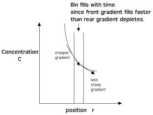
In the figure below, consider a concentration gradient across a bin. The gradient is steep on the front side of the bin and less steep at the rear side of the bin. Fick’s 1st Law pertains to the flux across the front and rear surfaces of the bin. Fick’s 2nd Law pertains to how the concentration within the bin will change with time which depends on the balance between the front flux and the rear flux. In this case, the bin will fill with time because the front flux due to the steep front gradient fills the bin faster than the rear flux with the less steep gradient empties the bin. Although the gradient ¶C/¶r is negative at both front and rear surfaces, the change in gradient as one moves from the front to the rear surface is positive.
1D diffusion
Consider a 1D diffusion problem along a position r (planar diffusion). Equation 2 is written for a 1D geometry:
![]() (eq.
3)
(eq.
3)
The numerical equivalent of this equation is written for C(ir) where ir is the index of the array C and denotes the central position of the irth bin, r(ir) = (ir – 0.5)dr. The expression for the change in C, dC, in one time step, dt, is:
 (eq.
4)
(eq.
4)
written using the MATLAB programming language:
dC(ir) = dt*alpha/dr^2*(C(ir+1) – 2*C(ir) + C(ir-1)); (eq. 5)
and the update of C(i) after one time step of diffusion is accomplished by:
C(ir) = C(ir) + dC(ir); (eq. 6)
2D diffusion
Consider 2D diffusion using cylindrical coordinates, radial position r and depth z. Equation 2 is written in cylindrical coordinates as:
![]() (eq.
7)
(eq.
7)
which can be written for numerical calculation in terms of C(iz,ir), where z =(iz – 0.5) dz and r = (ir – 0.5)dr, to yield:
 (eq.
8)
(eq.
8)
which for the case of uniform diffusivity, a, can be simplified to:
 (eq.
9)
(eq.
9)
Boundary conditions
Equation 9 is used for updating the bin C(iz,ir). However, when the indices (iz-1) or (ir-z) are applied to the first or last bin of the grid of the problem, one encounters a boundary. A simple boundary condition is an “insulating boundary” which is mimiced by assigning the value of the bin just outside the boundary the same value as the last bin inside the boundary. In other words, there is no gradient between the bins just inside and just outside the boundary. Hence, there is not net flux according to Fick’s 1st Law. However, Fick’s 2nd Law can still move flux into this last bin inside the boundary.
In the MATLAB program listed at the end of these notes, an array of size of Nz rows and Nr columns, C(Nz,Nr), is created. The domain of the problem is confined to the array C(2:Nz-1, 2:Nr-1), while the bins outside the boundaries are assigned to the bins C(2:Nz-1, 1), C(2:Nz-1, Nr), C(1, 2:Nr-1), and C(Nz, 2:Nr-1). The bins C(1,1), C(1,Nr), C(Nz,1), and C(Nz,Nr) are not used. Hence, the boundary conditions are set to “insulating” by the statements:
% boundary conditions
for ir=2:Nr-1
C(1,ir)
= C(2,ir); %
INSULATING top surface
C(Nz,ir)
= C(Nz-1, ir); % INSULATING bottom surface
end
for iz=2:Nz-1
C(iz,1)
= C(iz,2); %
INSULATING central z-axis
C(iz,Nr)
= C(iz, Nr-1); % INSULATING outer radial surface
end
Then the program can operate on the grid using the statements:
% within grid
for ir=2:Nr-1
for
iz=2:Nz-1
F1
= (C(iz,ir+1) - C(iz,ir-1))/r(ir)/2/dr;
F2
= (C(iz,ir+1) - 2*C(iz,ir) + C(iz,ir-1))/dr^2;
F3
= (C(iz+1,ir) - 2*C(iz,ir) + C(iz-1,ir))/dz^2;
dC(iz,ir)
= dt*a*(F1 + F2 + F3);
end
end
The following figure illustrates the grid with solid circles denoting bins outside the boundary and open circles denoting bins inside the boundary within the grid of interest. The grid covers onlyt he positive r-axis, and the grid at negative r is a mirror image.
The figure below shows an example of a simulation of the time-resolved response to a laser pulse. The circle at about (z = 9, r = 0) indicates the position of the laser pulse at 302 ps after launch at position (0,0) as it moves downward. The laser pulse duration was dz/c = 10.8 ps at a fluence rate c(1 J/cm3) = 3x10¹⁰ W/cm2. As the photon propagates, it is attenuated by exp(–(ma + ms) c dt) where c is the speed of light, t is the current time, ma is the absorption coefficient and ms is the scattering coefficient and isotropic scattering is assumed. The amount of light removed from the pulse and deposited into the diffusion problem at the current laser pulse’s position is ms dt cCp where cCp equals the surviving fluence rate of the pulse.
MATLAB program for diffusion in cylindrical coordinates
%%%%%%
% fdrz.m %
%%%%%%
% fdrz.m
clear
warning off
makec2
%%%%%%%%%%%%%%%%%
% USER CHOICES
%%%%%%%%%%%%%%%%%
Nr =
20; % number of bins
Nz =
2*Nr;
mua =
0.3; % [cm^-1]
musp = 10;
% [cm^-1]
b
= 0.1; % stability factor
%%%%%%%%%%%%%%%%%
%%%%%%%%%%%%%%%%%
mutp = mua + musp; % [cm^-1]
D
= 1/(mua + musp)/3;
c
= 3e10; % [cm/s]
a
= c*D % cm^2/s
dr =
a/b/c;% r bin size
dz =
dr; % z bin size
%%%% Set up arrays
C
= zeros(Nz,Nr); % array for photon concentration
dC =
zeros(Nz,Nr); % array for incremental concentration per timestep
W
= zeros(Nz-2, 2*(Nr-2));
rmax = (Nr-2)*dr;
zmax = (Nz-2)*dz;
z((1:Nz)',1) = dz*((1:Nz)' - 1.5); % rows at z
r((1:Nr)',1) = dr*((1:Nr)' - 1.5); % columns at r
rw =
(-rmax:dr:rmax);
zw =
(0:dz:zmax)';
dt =
b*dr^2/a; % time step [s]
disp(sprintf('dt = %5.3f ps', dt*1e12))
%%% draw grid
figure(1);clf
set(figure(1), 'position', [200 30 800 700])
plot([0 0],[0 zmax],'c-')
hold on
for ir=2:Nr-1
for
iz=1:Nz
plot(
[r(ir)+dr/2, r(ir)+dr/2], [-dz zmax+dz], 'c-')
plot(-[r(ir)+dr/2,
r(ir)+dr/2], [-dz zmax+dz], 'c-')
end
end
for iz=2:Nz-1
for
ir=1:Nr
plot([-rmax-dr
rmax+dr], [z(iz)+dz/2, z(iz)+dz/2], 'c-')
plot(r(ir),
z(iz),'ro')
end
end
plot([-rmax rmax rmax -rmax -rmax], [0 0 zmax zmax
0],'k-')
% domain of computation
plot([0 0],[0 zmax],'k-')
axis([-rmax rmax -dz zmax]*1.1)
axis ij
set(gca,'fontsize',24)
xlabel('r [cm]')
ylabel('z [cm]')
% boundary conditions
for ir=2:Nr-1
plot(r(ir),z(1),
'ro','markerfacecolor','r')
plot(r(ir),z(Nz),
'ro','markerfacecolor','r')
end
for iz=2:Nz-1
plot(r(1),z(iz),
'ro','markerfacecolor','r')
plot(r(Nr),z(iz),
'ro','markerfacecolor','r')
end
%%%%%%%%%%% INITIALIZE %%%%%%%%%%%%%%%%%
C(:,:) = 0;
Co
= 1; % [J/cm^3]
photon energy concentration of laser pulse
Eo
= c*Co; % [W/cm^2] irradiance of laser
C(2,2) = musp*dt*Eo;
% concentration of light scattered
in first time step
% laser pulse duration matches
time step dt
Cp
= Co*exp(-mutp*c*dt);
% photon energy concentration
remaining in laser pulse
disp(sprintf('Eo = %5.3e [W/cm2]', Eo))
time = 0;
drawC
plot([0 0],[-zmax*.7 0],'r-','linewidth',3)
text(rmax/10,-zmax/2,'Launch pulse of
light','fontsize',24)
pause(1)
i = 0;
%%%%%%%%%%%%%%%%% CYCLE %%%%%%%%%%%%%%%%%
while (time <= 10e-9)
i
= i + 1;
time
= time + dt;
% C(1,1), C(1,N), C(N,1), and C(N,N) not used
% boundary conditions
for ir=2:Nr-1
C(1,ir) = C(2,ir); % INSULATING top surface
C(Nz,ir)
= C(Nz-1, ir); % INSULATING bottom surface
end
for iz=2:Nz-1
C(iz,1) = C(iz,2); % INSULATING central z-axis
C(iz,Nr)
= C(iz, Nr-1); % INSULATING outer radial surface
end
% within volume
for ir=2:Nr-1
for
iz=2:Nz-1
F1
= (C(iz,ir+1) - C(iz,ir-1))/r(ir)/2/dr;
F2
= (C(iz,ir+1) - 2*C(iz,ir) + C(iz,ir-1))/dr^2;
F3
= (C(iz+1,ir) - 2*C(iz,ir) + C(iz-1,ir))/dz^2;
dC(iz,ir)
= dt*a*(F1 + F2 + F3);
end
end
% Update C
C = C + dC;
drawC
% Draw photon pulse
zs = time*c;
plot(0,zs,'ro','markerfacecolor','y',
'markersize',12,'linewidth',3)
% Scatter light from pulse
if zs<=zmax
ii
= round(zs/dz) + 2;
C(ii,2)
= C(ii,2) + musp*dt*c*Cp;
Cp
= Cp*exp(-mutp*c*dt);
end
drawnow
end % while
%%%%%%%%%%%%% end CYCLE %%%%%%%%%%%%%%%%%
%%%%%%%%%%%%%%%%
%% drawC.m %%%%
%%%%%%%%%%%%%%%%
% draw W map
% Create W from C for +/- r vs z
% Plot in Figure 2
figure(2);clf
set(figure(2), 'position', [10 100 1000 700])
maxC
= max(max(C));
temp
= C(2:Nz-1, 2:Nr-1)*exp(-mua*c*time)/Co;
Nw = 2*(Nr-2);
W(:,Nw/2+1:Nw)
= temp;
W(:,Nw/2:-1:1)
= temp;
imagesc(rw,zw,log10(W),[-12 0])
%imagesc(rw,zw,W,[0.999 1.001])
%imagesc(rw,zw,W, [0 1])
colorbar
colormap(c2)
axis('square')
set(gca,'fontsize',24)
set(colorbar,'fontsize',24)
text(rmax,-zmax*0.05,'log_1_0(C/U_0)','fontsize',24)
xlabel('r [cm]')
ylabel('z [cm]')
axis([-rmax rmax 0 zmax])
if time<1000e-12
title(sprintf('time
= %5.0f [ps]',time*1e12),'fontsize',36)
else
title(sprintf('time
= %5.3f [ns]',time*1e9),'fontsize',36)
end
hold on